Sensitivity to tau

Code

library(tidyverse)
library(targets)
tar_source()
tar_load(exp1_data_agg)

In the current draft (May 12th), Eda modelled the data by ignoring the first chunk when calculating the likelihood.

Here are the predictions using the parameters reported in the paper:

Code

start <- paper_params()

exp1_data_agg$pred <- predict(start, data = exp1_data_agg, group_by = c("chunk", "gap"))

exp1_data_agg |>
  ggplot(aes(x = gap, y = p_correct, color = chunk)) +
  geom_point() +
  geom_line() +
  geom_line(aes(y = pred), linetype = "dashed") +
  facet_wrap(~itemtype)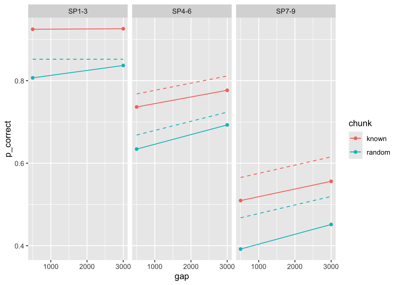

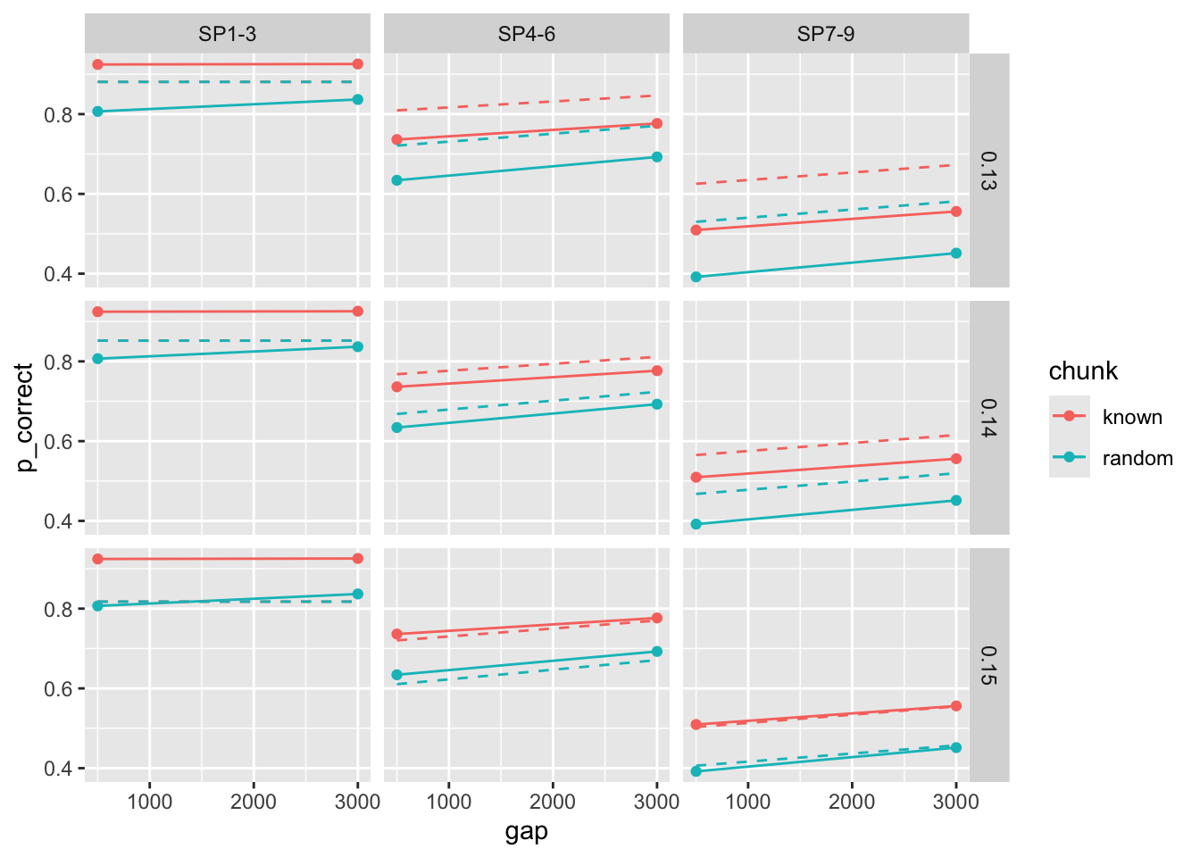
Strangely, there is a mismatch between these results and what is reported in the paper.

This is because the predictions are extremely sensitive to small changes in tau:

Code

params <- list(start, start, start)
params[[2]][["tau"]] <- 0.15
params[[3]][["tau"]] <- 0.13


overall_deviance(params[[1]], exp1_data_agg, by = c("chunk", "gap"), exclude_sp1 = TRUE)

[1] 116.5524

Code

overall_deviance(params[[2]], exp1_data_agg, by = c("chunk", "gap"), exclude_sp1 = TRUE)

[1] 38.11554

Code

overall_deviance(params[[3]], exp1_data_agg, by = c("chunk", "gap"), exclude_sp1 = TRUE)

[1] 395.7678

Code

exp1_data_agg$pred2 <- predict(params[[2]], data = exp1_data_agg, group_by = c("chunk", "gap"))
exp1_data_agg$pred3 <- predict(params[[3]], data = exp1_data_agg, group_by = c("chunk", "gap"))

exp1_data_agg |>
  pivot_longer(cols = starts_with("pred"), names_to = "tau", values_to = "pred") |>
  mutate(tau = case_when(
    tau == "pred" ~ "0.14",
    tau == "pred2" ~ "0.15",
    tau == "pred3" ~ "0.13"
  )) |>
  ggplot(aes(x = gap, y = p_correct, color = chunk)) +
  geom_point() +
  geom_line() +
  geom_line(aes(y = pred), linetype = "dashed") +
  facet_grid(tau ~ itemtype)