Extra primacy parameter

TODO: Clean-up this notebook

library(tidyverse)
library(targets)
tar_source()
tar_load(c(exp3_data_agg, exp3_data))

Define new model likelihood

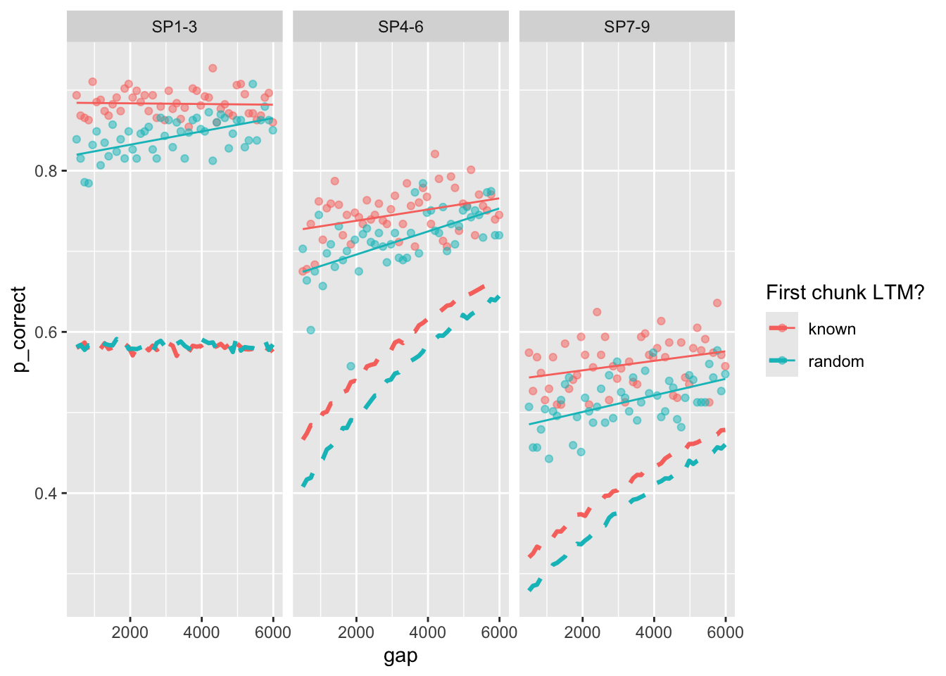
One example fit:

set.seed(25)
fit <- estimate_model(c(start_fun(), prim_prop = rbeta(1, 5, 2)), exp3_data_agg, version = 2, exclude_sp1 = T)
kableExtra::kable(optimfit_to_df(fit))

prop	prop_ltm	rate	gain	tau	prim_prop	deviance	convergence
0.129707	0.5184667	0.1597853	42.70181	0.089936	0.9305835	760.8202	0

exp3_data_agg$pred <- predict(fit, exp3_data_agg, group_by = c("chunk", "gap"))

exp3_data_agg |>
  ggplot(aes(x = gap, y = p_correct, color = chunk)) +
  geom_point(alpha = 0.5) +
  stat_smooth(method = "lm", se = FALSE, linewidth = 0.5) +
  geom_line(aes(y = pred), linetype = "dashed", linewidth = 1.1) +
  scale_color_discrete("First chunk LTM?") +
  facet_wrap(~itemtype)

Run the estimation 100 times with different starting values:

set.seed(18)
fits <- run_or_load(
  {
    res <- replicate(
      n = 100,
      expr = estimate_model(
        c(start_fun(), prim_prop = rbeta(1, 5, 2)),
        exp3_data_agg,
        version = 2, exclude_sp1 = T
      ),
      simplify = FALSE
    )
    res <- do.call(rbind, lapply(res, optimfit_to_df))
    arrange(res, deviance)
  },
  file = "output/exp3_fits_100_prop_primacy.rds"
)

Refine the fits with a second pass starting from the best fit:

fits_refined <- run_or_load(
  {
    res <- apply(fits, 1, function(x) {
      fit <- estimate_model(x, exp3_data_agg, version = 2, exclude_sp1 = T)
      optimfit_to_df(fit)
    })
    do.call(rbind, res)
  },
  file = "output/exp3_fits_100_prop_primacy_refined.rds"
)
fits_refined$deviance <- 2 * fits_refined$deviance

Print fits sorted by deviance:

kableExtra::kable(arrange(fits_refined, deviance))

prop	prop_ltm	rate	gain	tau	prim_prop	deviance	convergence
0.0830018	0.5354440	0.1521677	100.00000	0.0664134	0.9592183	1520.717	0
0.0830345	0.5354821	0.1522194	99.92881	0.0664355	0.9592133	1520.717	0
0.0827561	0.5303713	0.1540288	99.99304	0.0661689	0.9585271	1520.720	0
0.0833021	0.5326726	0.1534809	98.99042	0.0665430	0.9585757	1520.723	0
0.0836369	0.5354833	0.1524269	98.53729	0.0668022	0.9588923	1520.724	0
0.0838078	0.5349846	0.1527897	98.13969	0.0669035	0.9587414	1520.726	0
0.0839589	0.5352356	0.1523192	97.77404	0.0669837	0.9586211	1520.728	0
0.0840183	0.5344278	0.1528843	97.58774	0.0670162	0.9585227	1520.729	0
0.0840788	0.5337896	0.1528134	97.48065	0.0670620	0.9585533	1520.729	0
0.0843323	0.5352119	0.1524255	96.99083	0.0672207	0.9584937	1520.731	0
0.0844863	0.5384292	0.1511989	96.96959	0.0673687	0.9588990	1520.732	0
0.0841521	0.5333316	0.1531871	97.06339	0.0670524	0.9581341	1520.733	0
0.0850234	0.5387903	0.1513496	95.74477	0.0676811	0.9585429	1520.738	0
0.0854952	0.5374167	0.1511926	94.65133	0.0679400	0.9581097	1520.744	0
0.0853425	0.5370373	0.1515787	94.77365	0.0678094	0.9579259	1520.744	0
0.0854451	0.5350333	0.1525429	94.50061	0.0678727	0.9577814	1520.745	0
0.0857269	0.5368538	0.1515001	94.18233	0.0680980	0.9581038	1520.746	0
0.0872424	0.5390619	0.1510209	91.40748	0.0690687	0.9577849	1520.763	0
0.0878679	0.5354037	0.1524971	89.87321	0.0693818	0.9569372	1520.771	0
0.0880266	0.5353644	0.1539354	89.55011	0.0694815	0.9567853	1520.778	0
0.0884297	0.5360268	0.1513224	88.72862	0.0696856	0.9565830	1520.779	0
0.0878443	0.5251040	0.1565616	89.02264	0.0691813	0.9553297	1520.786	0
0.0892337	0.5399017	0.1496270	87.49761	0.0702117	0.9566977	1520.788	0
0.0896874	0.5467911	0.1466649	86.80853	0.0704719	0.9567592	1520.802	0
0.0915173	0.5403781	0.1506760	83.44070	0.0715516	0.9554777	1520.814	0
0.0915863	0.5467830	0.1481750	83.97125	0.0717513	0.9567280	1520.815	0
0.0907884	0.5516159	0.1462604	85.63544	0.0713531	0.9578251	1520.816	0
0.0904884	0.5308324	0.1531446	84.52523	0.0708115	0.9548965	1520.819	0
0.0921162	0.5379638	0.1511176	82.15251	0.0718255	0.9546897	1520.824	0
0.0934299	0.5461201	0.1483120	80.77434	0.0727898	0.9556430	1520.837	0
0.0936599	0.5373178	0.1509119	79.91900	0.0728257	0.9546394	1520.847	0
0.0934048	0.5373752	0.1522977	79.64859	0.0724489	0.9532476	1520.856	0
0.0954108	0.5338564	0.1530252	76.62310	0.0736285	0.9523789	1520.874	0
0.0964956	0.5497604	0.1470154	76.30653	0.0746150	0.9547932	1520.879	0
0.0917041	0.5584003	0.1470930	83.85527	0.0717872	0.9566873	1520.882	0
0.0973273	0.5302367	0.1539601	73.54802	0.0746042	0.9507225	1520.911	0
0.0987585	0.5460551	0.1491697	72.64034	0.0757628	0.9528200	1520.913	0
0.0987959	0.5381743	0.1510308	71.89543	0.0755197	0.9509666	1520.921	0
0.1007429	0.5473097	0.1478690	70.29082	0.0769701	0.9526443	1520.941	0
0.1031380	0.5365476	0.1515734	66.21486	0.0778125	0.9484016	1520.993	0
0.1041868	0.5425277	0.1497028	65.23047	0.0784592	0.9486410	1521.005	0
0.1041107	0.5585138	0.1426450	66.85880	0.0790617	0.9531637	1521.005	0
0.1052323	0.5522870	0.1466097	65.03940	0.0794905	0.9512479	1521.012	0
0.1032888	0.5270420	0.1553102	65.66822	0.0777932	0.9473241	1521.014	0
0.1050829	0.5429193	0.1493026	64.45731	0.0790327	0.9487062	1521.016	0
0.1055747	0.5453514	0.1495319	64.38901	0.0795725	0.9500933	1521.017	0
0.1057176	0.5363009	0.1519290	63.21499	0.0791567	0.9469873	1521.037	0
0.1056761	0.5328284	0.1528260	63.19574	0.0791423	0.9469534	1521.040	0
0.1095031	0.5597043	0.1427385	60.18882	0.0814623	0.9482292	1521.102	0
0.1038245	0.5178414	0.1606086	64.11113	0.0776493	0.9440227	1521.108	0
0.1112165	0.5405131	0.1513658	57.83141	0.0821252	0.9451479	1521.121	0
0.1139487	0.5665163	0.1408282	56.79748	0.0842963	0.9495305	1521.163	0
0.1150464	0.5620415	0.1424970	55.49423	0.0846745	0.9478959	1521.174	0
0.1104956	0.5844357	0.1330230	61.23827	0.0830523	0.9550584	1521.176	0
0.1150277	0.5707915	0.1394673	56.13136	0.0850230	0.9502024	1521.195	0
0.1168787	0.5563987	0.1475113	53.57138	0.0854354	0.9456710	1521.224	0
0.1170302	0.5467398	0.1477255	52.79237	0.0850381	0.9430341	1521.225	0
0.1190151	0.5745878	0.1375233	52.76130	0.0870007	0.9487474	1521.265	0
0.1180843	0.5374202	0.1543369	51.51058	0.0853142	0.9404624	1521.282	0
0.1206378	0.5369294	0.1526183	49.75313	0.0867212	0.9404126	1521.311	0
0.1222813	0.5450775	0.1484505	48.58462	0.0874118	0.9398335	1521.338	0
0.1219608	0.5950076	0.1293583	51.47250	0.0890850	0.9520846	1521.387	0
0.1258652	0.5543236	0.1449665	46.47660	0.0893696	0.9402240	1521.393	0
0.1261358	0.5512622	0.1469249	46.15517	0.0893986	0.9393450	1521.405	0
0.1229203	0.6004439	0.1274795	51.09406	0.0898015	0.9532568	1521.437	0
0.1253455	0.5347543	0.1524909	45.93500	0.0884188	0.9358299	1521.453	0
0.1096435	0.6245279	0.1157842	65.14104	0.0838056	0.9644263	1521.465	0
0.1291902	0.5698808	0.1404231	44.52248	0.0909739	0.9401136	1521.507	0
0.1316542	0.5861278	0.1329112	44.07969	0.0930474	0.9448045	1521.528	0
0.1320240	0.5487744	0.1460666	42.47430	0.0920422	0.9368930	1521.552	0
0.1407647	0.5726243	0.1378135	38.67907	0.0966723	0.9386590	1521.727	0
0.1410802	0.5921934	0.1299198	39.08275	0.0972915	0.9421512	1521.746	0
0.1416289	0.5584553	0.1449145	37.55499	0.0961602	0.9331385	1521.772	0
0.1442493	0.5817889	0.1357689	37.16069	0.0981666	0.9379234	1521.805	0
0.1485820	0.5506684	0.1476578	34.44050	0.0989464	0.9297136	1521.974	0
0.1335032	0.4896621	0.1771724	40.02027	0.0912584	0.9248692	1522.027	0
0.1508329	0.5659537	0.1397505	33.56548	0.0994088	0.9283791	1522.043	0
0.1464991	0.6365233	0.1119736	38.25589	0.1015555	0.9525763	1522.066	0
0.1570901	0.5720074	0.1369226	31.39721	0.1020279	0.9277262	1522.192	0
0.1578781	0.5796311	0.1354878	31.28607	0.1025839	0.9289186	1522.195	0
0.1557528	0.5623220	0.1426612	31.36372	0.1005411	0.9230903	1522.254	0
0.1615952	0.5661500	0.1440328	29.91051	0.1040553	0.9264082	1522.330	0
0.1625162	0.5859924	0.1360934	29.80458	0.1043471	0.9275039	1522.355	0
0.1643793	0.6202930	0.1195451	30.34787	0.1072577	0.9396434	1522.388	0
0.1628606	0.6659198	0.1026569	32.71971	0.1100000	0.9576486	1522.606	0
0.1673065	0.5570623	0.1476521	27.42337	0.1035436	0.9131497	1522.795	0
0.1494665	0.7064391	0.0870326	40.84013	0.1073822	0.9772426	1522.822	0
0.1757971	0.5737036	0.1355153	25.60590	0.1074592	0.9172798	1522.859	0
0.1237810	0.7275594	0.0803559	60.88937	0.0958362	0.9892582	1522.916	0
0.1478485	0.7136234	0.0842819	42.33303	0.1072880	0.9809562	1522.918	0
0.1508772	0.7128888	0.0843160	40.69104	0.1086132	0.9801147	1522.946	0
0.1641892	0.5166694	0.1581206	27.52562	0.1009010	0.9058324	1522.977	0
0.1454702	0.7272316	0.0801023	44.59122	0.1069657	0.9859114	1523.054	0
0.1560018	0.7256169	0.0812223	39.04160	0.1118570	0.9840110	1523.160	0
0.1008613	0.7540632	0.0701410	95.94044	0.0832805	0.9999999	1523.350	0
0.1500814	0.7543605	0.0712736	44.53389	0.1115246	0.9976890	1523.548	0
0.2012512	0.6942274	0.0925222	22.99875	0.1245127	0.9570987	1523.700	0
0.1954065	0.5381045	0.1690204	21.11082	0.1135602	0.9050614	1524.333	0
0.2222245	0.7091319	0.0886436	19.79598	0.1324736	0.9621327	1524.418	0
0.2420613	0.7426193	0.0755768	17.80195	0.1411300	0.9779758	1525.069	0

Not as much variance as I thought there would be. Let’s limit to the fits within 2 deviance units of the best fit:

Here is the distribution of parameter values that are within 2 deviance units of the best fit:

best_fits <- filter(fits_refined, deviance < min(deviance) + 2)

best_fits |>
  select(prop:prim_prop) |>
  pivot_longer(cols = everything(), names_to = "parameter", values_to = "value") |>
  ggplot(aes(x = value)) +
  geom_histogram(bins = 30) +
  facet_wrap(~parameter, scales = "free") +
  theme_pub()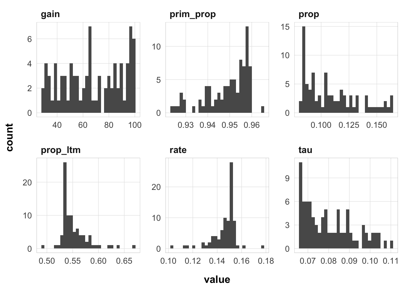

Here is the plot of the best fitting model:

best_fit <- estimate_model(unlist(best_fits[1, 1:6]), exp3_data_agg, version = 2, exclude_sp1 = T)
exp3_data_agg$pred <- predict(best_fit, exp3_data_agg, group_by = c("chunk", "gap"))

exp3_data_agg |>
  ggplot(aes(x = gap, y = p_correct, color = chunk)) +
  geom_point(alpha = 0.5) +
  stat_smooth(method = "lm", se = FALSE, linewidth = 0.5) +
  geom_line(aes(y = pred), linetype = "dashed", linewidth = 1.1) +
  scale_color_discrete("First chunk LTM?") +
  facet_wrap(~itemtype)

`geom_smooth()` using formula = 'y ~ x'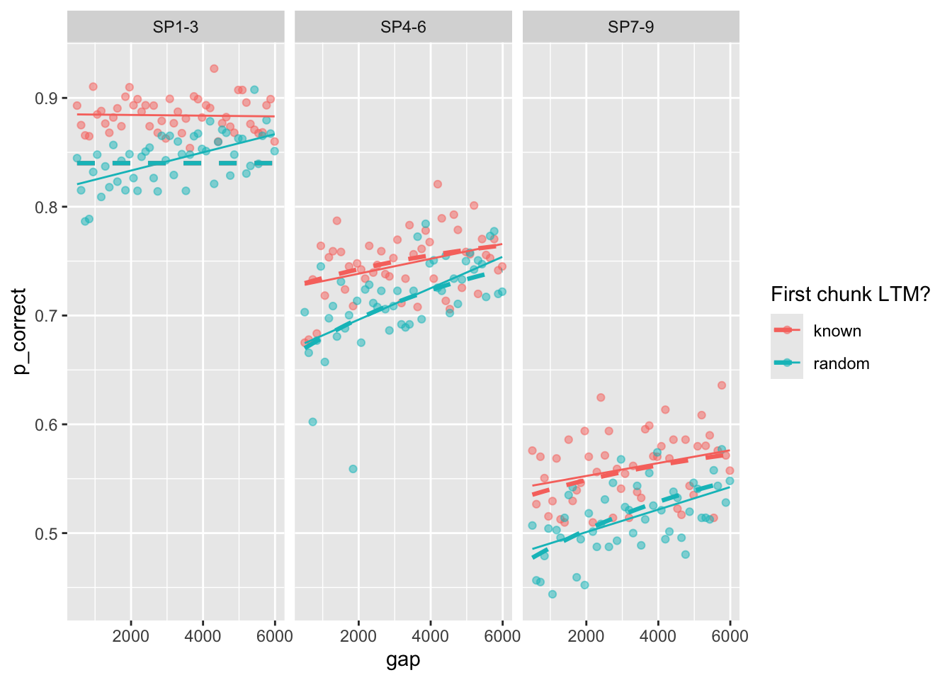

and the parameter estimates:

kableExtra::kable(t(as.data.frame(best_fit$par)))

	prop	prop_ltm	rate	gain	tau	prim_prop
x	0.0827601	0.5305627	0.1540501	99.99801	0.0661733	0.958538

with this rate, the resource recovery over time looks like this:

resources <- function(R, rate, time, r_max = 1) {
  (r_max - R) * (1 - exp(-rate * time))
}

time <- seq(0, 20, 0.1)
tibble(time = time, resources = resources(0, best_fits[1, ]$rate, time)) |>
  ggplot(aes(x = time, y = resources)) +
  geom_line() +
  theme_pub()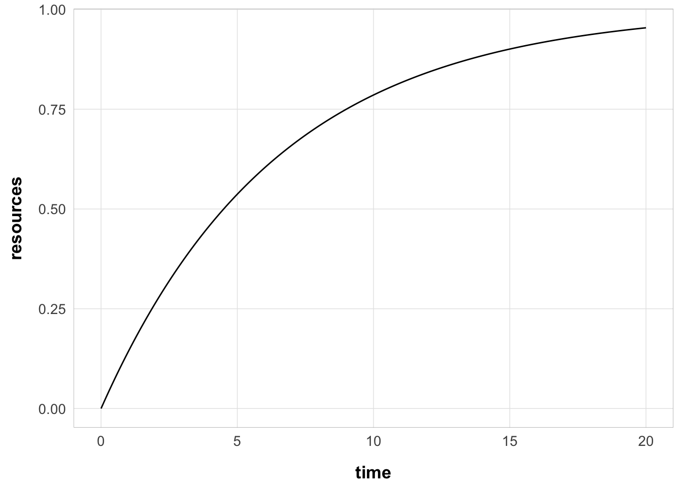

with 50% of the resource recovered after 4.5 seconds

and 25% of the resource recovered after 1.87 seconds

Simulate full trial sequences

With recovery during entire recall period

Calculate the total recall period duration on each trial:

total_rts <- exp3_data |>
  group_by(id, trial) |>
  summarize(total_recall_duration = sum(rt) + 9 * 0.2 + 1)

`summarise()` has grouped output by 'id'. You can override using the `.groups` argument.

hist(total_rts$total_recall_duration, breaks = 30, col = "grey", border = "white", xlab = "Total recall period duration (s.)", main = "")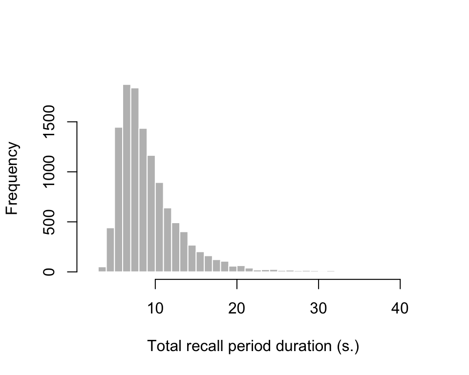

Create the trial structure for the simulation:

exp3_trial_str <- run_or_load({
  exp3_data |>
  group_by(id, trial) |>
  do({
    aggregate_data(.)
  })
}, file = "output/exp3_trial_structure.rds")

exp3_trial_str <- left_join(exp3_trial_str, total_rts) |> 
  mutate(ISI = ifelse(itemtype == "SP7-9", total_recall_duration, ISI),
         ser_pos = case_when(
          itemtype == "SP1-3" ~ 1,
          itemtype == "SP4-6" ~ 2,
          itemtype == "SP7-9" ~ 3
         ))

Run the model without resetting the resource at the start of each trial:

serial_recall_full <- function(
    setsize, ISI = rep(0.5, setsize), item_in_ltm = rep(TRUE, setsize), ser_pos = 1:setsize, 
    prop = 0.2, prop_ltm = 0.5, tau = 0.15, gain = 25, rate = 0.1, prim_prop = 1,
    r_max = 1, lambda = 1, growth = "linear") {
  R <- r_max
  p_recall <- vector("numeric", length = setsize)
  prop_ltm <- ifelse(item_in_ltm, prop_ltm, 1)

  for (item in 1:setsize) {
    # strength of the item and recall probability
    strength <- (prop * R)^lambda * prim_prop^(ser_pos[item] - 1)
    p_recall[item] <- 1 / (1 + exp(-(strength - tau) * gain))

    # amount of resources consumed by the item
    r_cost <- strength^(1 / lambda) * prop_ltm[item]
    R <- R - r_cost

    # recover resources
    R <- switch(growth,
      "linear" = min(r_max, R + rate * ISI[item]),
      "asy" = R + (r_max - R) * (1 - exp(-rate * ISI[item]))
    )
  }

  p_recall
}

subj1 <- exp3_trial_str |>
  filter(id == 44125)

Here it is for one example subject:

subj1$pred <- serial_recall_full(
  setsize = nrow(subj1),
  ISI = subj1$ISI,
  item_in_ltm = subj1$item_in_ltm,
  ser_pos = subj1$ser_pos,
  prop = best_fit$par["prop"],
  prop_ltm = best_fit$par["prop_ltm"],
  tau = best_fit$par["tau"],
  gain = best_fit$par["gain"],
  rate = best_fit$par["rate"],
  prim_prop = best_fit$par["prim_prop"],
  growth = "asy"
)

subj1 |>
  ungroup() |>
  mutate(absolute_position = 1:n()) |>
  ggplot(aes(x = absolute_position, y = pred)) +
  geom_point() +
  geom_line() +
  theme_pub()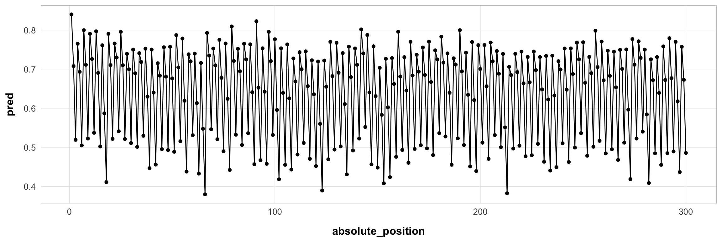

Same, but collapsed over serial position (one value per trial):

subj1 |>
  ungroup() |>
  ggplot(aes(x = trial, y = pred)) +
  stat_summary(geom = "point") +
  geom_smooth() +
  theme_pub()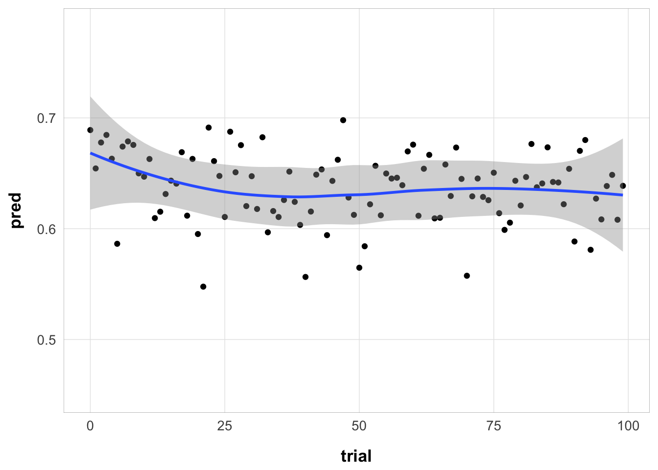

Now simulate the full dataset:

sim_no_reset_full <- function(data, best_fit) {
  data |>
    group_by(id) |>
    mutate(pred = serial_recall_full(
      setsize = n(),
      ISI = ISI,
      item_in_ltm = item_in_ltm,
      ser_pos = ser_pos,
      prop = best_fit$par["prop"],
      prop_ltm = best_fit$par["prop_ltm"],
      tau = best_fit$par["tau"],
      gain = best_fit$par["gain"],
      rate = best_fit$par["rate"],
      prim_prop = best_fit$par["prim_prop"],
      growth = "asy"
    ))
}

full_sim <- sim_no_reset_full(exp3_trial_str, best_fit)

ggplot(full_sim, aes(x = trial, y = pred)) +
  stat_summary() +
  geom_smooth() +
  theme_pub()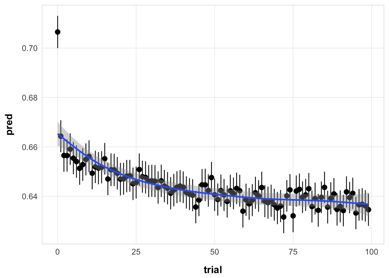

Yes, the model predicts worsening performance over trials, but the effect is miniscule.

Plot the original predictions recomputed with the full trial-by-trial model:

full_sim |>
  group_by(chunk, gap, itemtype) |>
  summarize(pred = mean(pred),
            p_correct = mean(p_correct)) |>
  ggplot(aes(x = gap, y = p_correct, color = chunk)) +
  geom_point(alpha = 0.5) +
  stat_smooth(method = "lm", se = FALSE, linewidth = 0.5) +
  geom_line(aes(y = pred), linetype = "dashed", linewidth = 1.1) +
  scale_color_discrete("First chunk LTM?") +
  facet_wrap(~itemtype)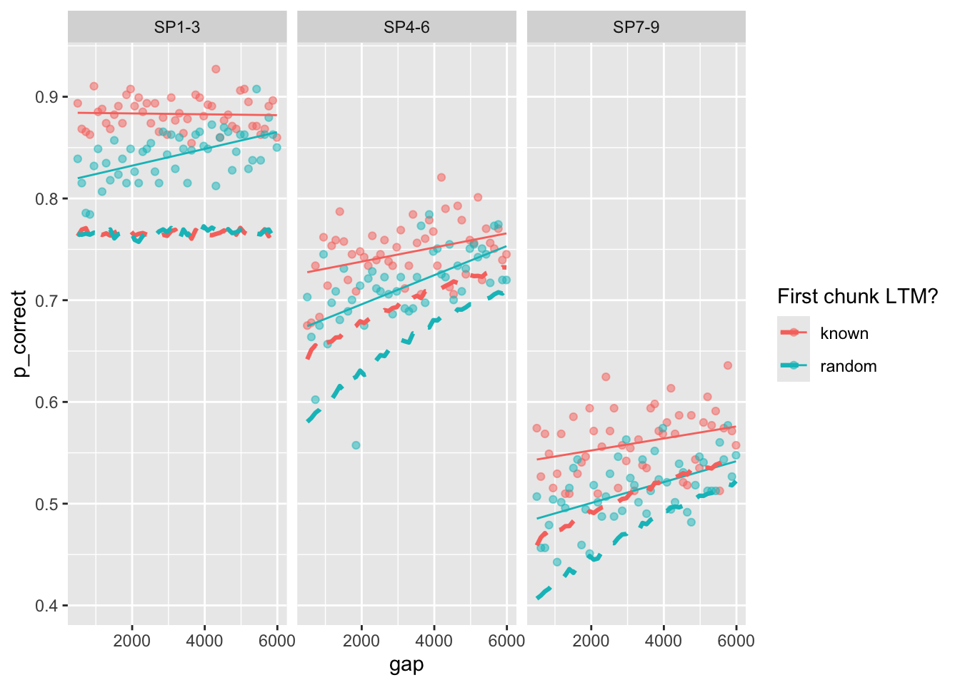

No recovery during recall, except during empty screens

exp3_trial_str <- run_or_load(
  {
    exp3_data |>
      group_by(id, trial) |>
      do({
        aggregate_data(.)
      })
  },
  file = "output/exp3_trial_structure.rds"
)


exp3_trial_str <- exp3_trial_str |>
  mutate(
    ISI = ifelse(itemtype == "SP7-9", 9 * 0.2 + 1, ISI),
    ser_pos = case_when(
      itemtype == "SP1-3" ~ 1,
      itemtype == "SP4-6" ~ 2,
      itemtype == "SP7-9" ~ 3
    )
  )

full_sim_v2 <- sim_no_reset_full(exp3_trial_str, best_fit)

ggplot(full_sim_v2, aes(x = trial, y = pred)) +
  stat_summary() +
  theme_pub()

No summary function supplied, defaulting to `mean_se()`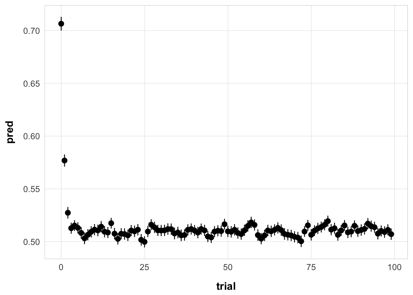

filter(full_sim_v2, id == 44125) |>
  mutate(absolute_position = 1:n()) |>
  ggplot(aes(x = absolute_position, y = pred)) +
  geom_point() +
  geom_line() +
  theme_pub()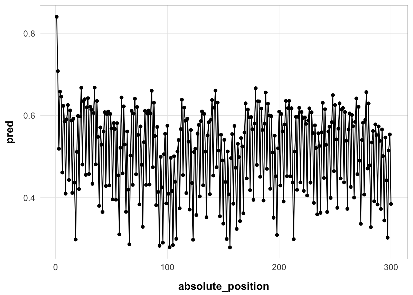

full_sim_v2 |>
  group_by(chunk, gap, itemtype) |>
  summarize(pred = mean(pred),
            p_correct = mean(p_correct)) |>
  ggplot(aes(x = gap, y = p_correct, color = chunk)) +
  geom_point(alpha = 0.5) +
  stat_smooth(method = "lm", se = FALSE, linewidth = 0.5) +
  geom_line(aes(y = pred), linetype = "dashed", linewidth = 1.1) +
  scale_color_discrete("First chunk LTM?") +
  facet_wrap(~itemtype)