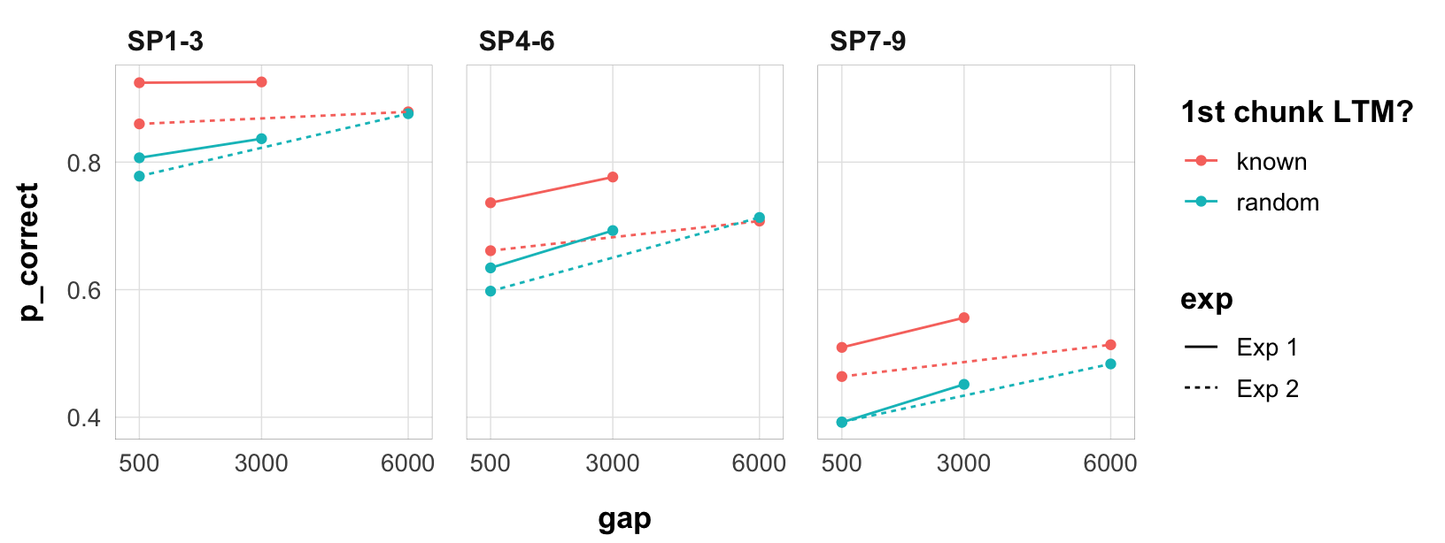
Overall performance is a bit lower in experiment 2, but not by much. Still, it might be an issue if trying to model the two experiments together. The effect size of the chunk is also smaller.
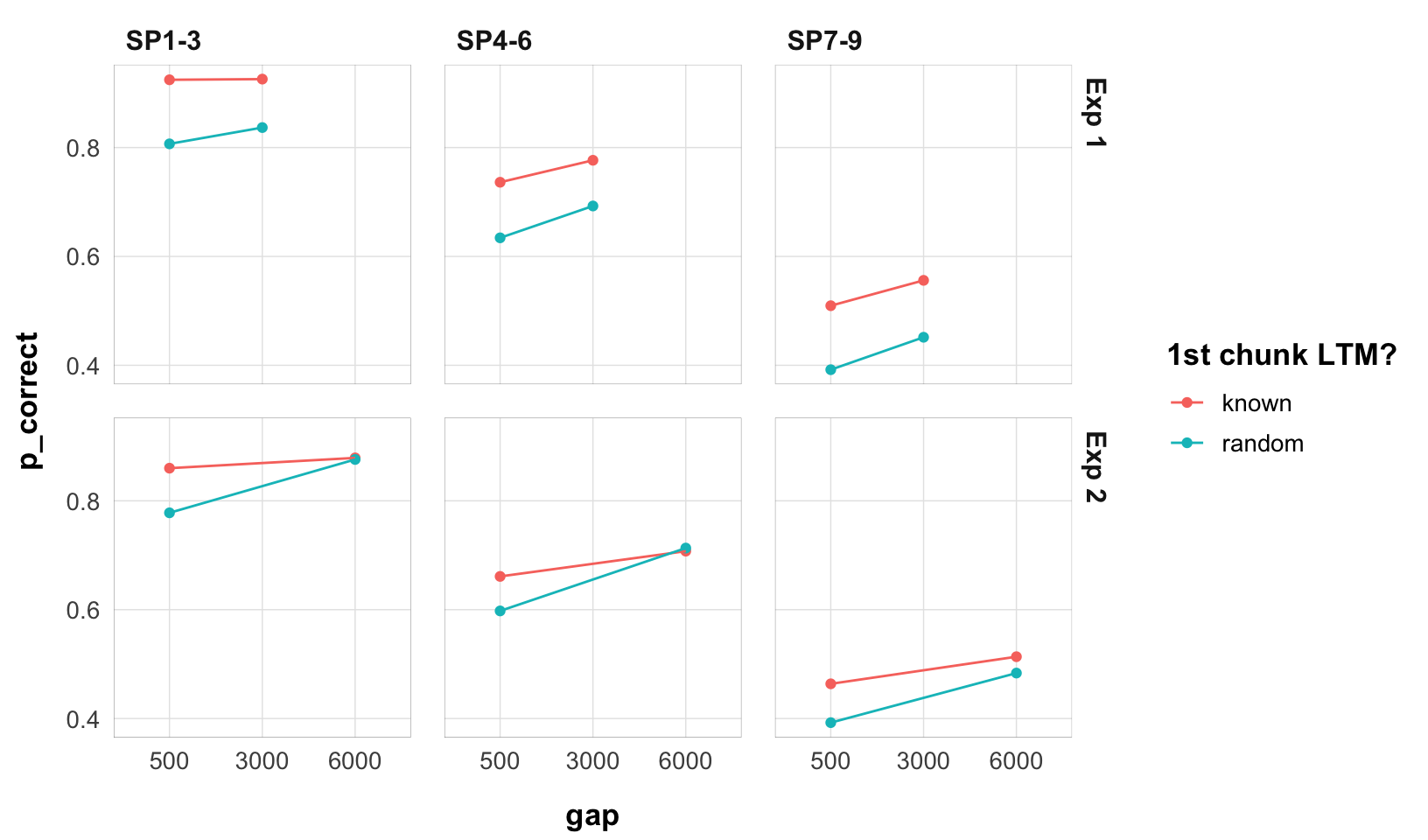
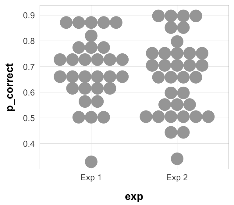
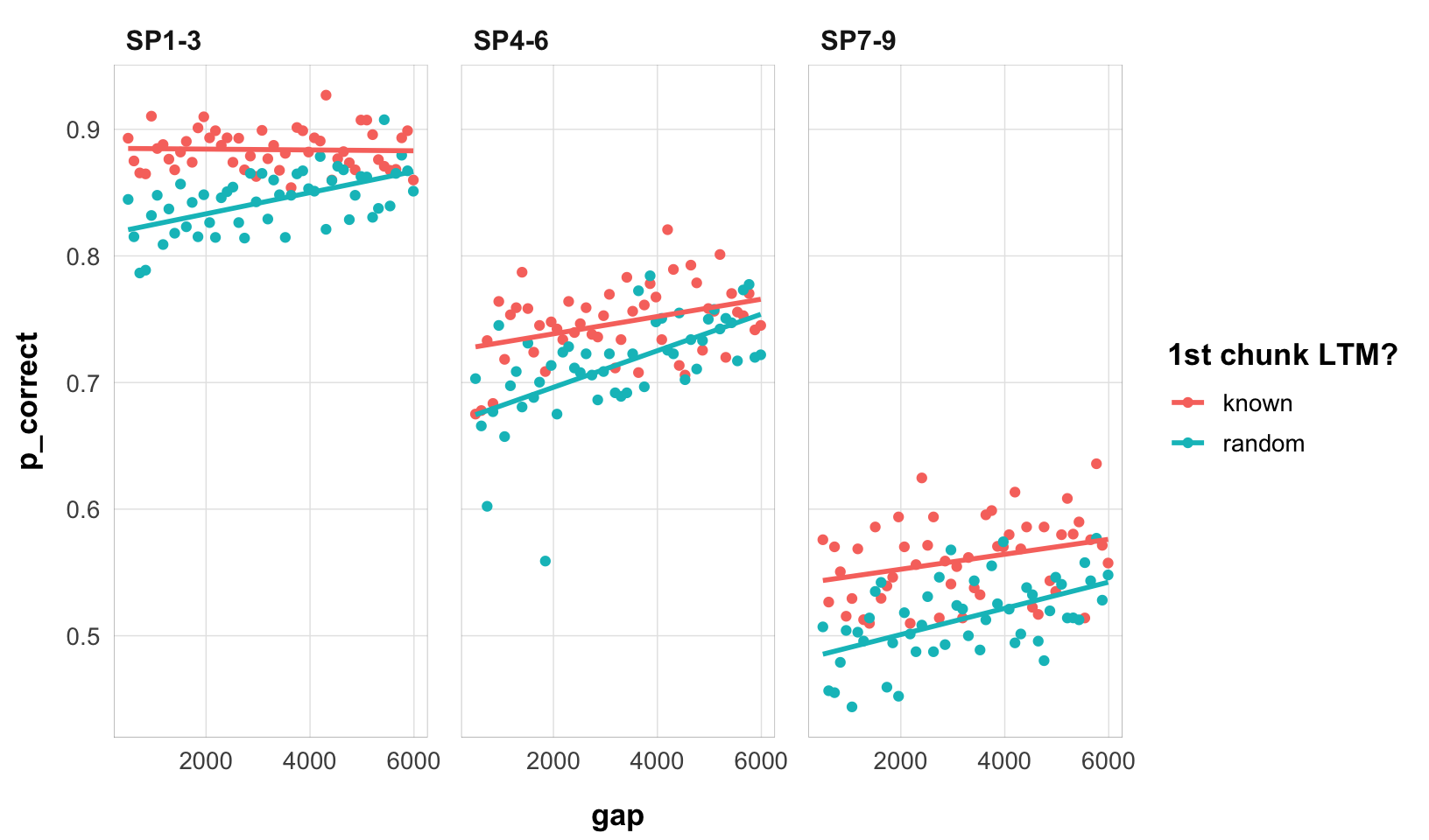
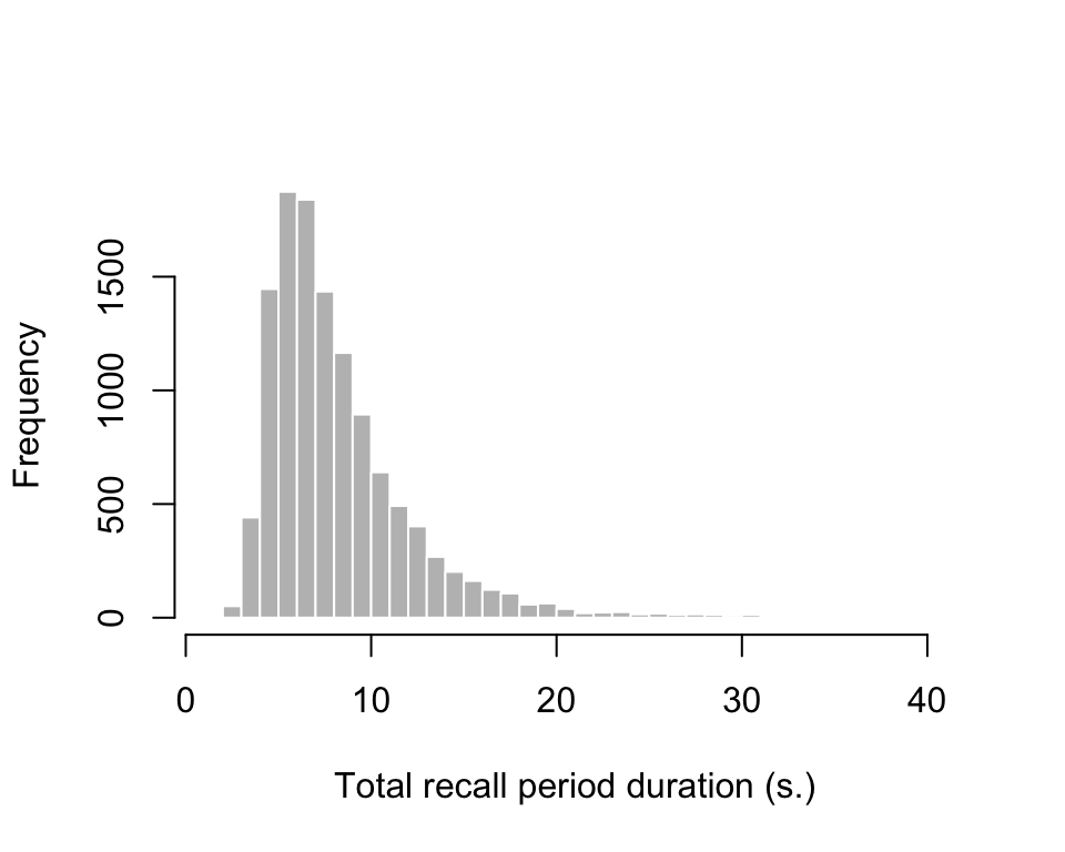
---title: "Exploratory data analysis"format: html---## Overview```{r}#| label: init#| message: falselibrary(tidyverse)library(targets)library(ggdist)tar_source()tar_load(c(exp1_data, exp2_data, exp1_data_agg, exp2_data_agg, exp3_data, exp3_data_agg))data_agg <-bind_rows(mutate(exp1_data_agg, exp ="Exp 1"),mutate(exp2_data_agg, exp ="Exp 2"))```Here I have a bunch of plots to help me understand the data for the later modeling.## Overall performance```{r}#| label: overall_performance_exp1#| fig-width: 8.5#| fig-height: 5data_agg |>mutate(gap =as.factor(gap)) |>ggplot(aes(gap, p_correct, color = chunk, group = chunk)) +geom_point() +geom_line() +scale_color_discrete("1st chunk LTM?") +facet_grid(exp ~ itemtype) +theme_pub()```Together to compare shared levels:```{r}#| label: overall_performance_exp1_shared_levels#| fig-width: 8.5#| fig-height: 3.2data_agg |>ggplot(aes(gap, p_correct, color = chunk, linetype = exp)) +geom_point() +geom_line() +scale_color_discrete("1st chunk LTM?") +scale_x_continuous(breaks =c(500, 3000, 6000)) +coord_cartesian(xlim =c(300, 6200)) +facet_wrap(~itemtype) +theme_pub()```Overall performance is a bit lower in experiment 2, but not by much. Still, it might be an issue if trying to model the two experiments together. The effect size of the chunk is also smaller.## Individual performance```{r}#| label: agg_data_subj#| message: falsedata_agg_subj <-bind_rows(mutate(exp1_data, exp ="Exp 1"),mutate(exp2_data, exp ="Exp 2")) |>group_by(id, exp) |>nest() |>mutate(data =map(data, aggregate_data)) |>unnest(data)```print overall accuracy for each subject:```{r}#| label: overall_accuracy#| fig-width: 4#| fig-height: 3.5#| message: falsedata_agg_subj |>group_by(exp, id) |>summarize(p_correct =mean(p_correct)) |>ggplot(aes(exp, p_correct)) +geom_dotsinterval(side ="both") +theme_pub()```## Experiment 3```{r}#| label: exp3_performance#| fig-width: 8.5#| fig-height: 5exp3_data_agg |>ggplot(aes(gap, p_correct, color = chunk, group = chunk)) +geom_point() +stat_smooth(method ="lm", se =FALSE) +scale_color_discrete("1st chunk LTM?") +facet_wrap(~itemtype) +theme_pub()```## Recall timesThis is the distribution of total recall period duration for experiment 3:```{r}#| label: recall_times#| fig-width: 5#| fig-height: 4total_rts <- exp3_data |>group_by(id, trial) |>summarize(total_recall_duration =sum(rt) +9*0.2) |>pluck("total_recall_duration")hist(total_rts, breaks =30, col ="grey", border ="white", xlab ="Total recall period duration (s.)", main ="")```