which can be simplified in the case of recovery starting from 0 to
\[
R(t) = 1 - e^{-r t}
\]
Klaus and I discussed the possibility that the recovery is linear, but the rate of recovery r is a random variable that varies over trials and individuals. Similarly to the evidence accumulation rate in the linear balistic accumulator models, at the aggregate level the recovery rate might be better modeled with the exponential recovery equation, even if the individual recovery is linear. In this notebook, I explore this idea further and derive analytical solutions for the average recovery over time under different assumptions about the distribution of r.
Linear recovery with a random variable rate
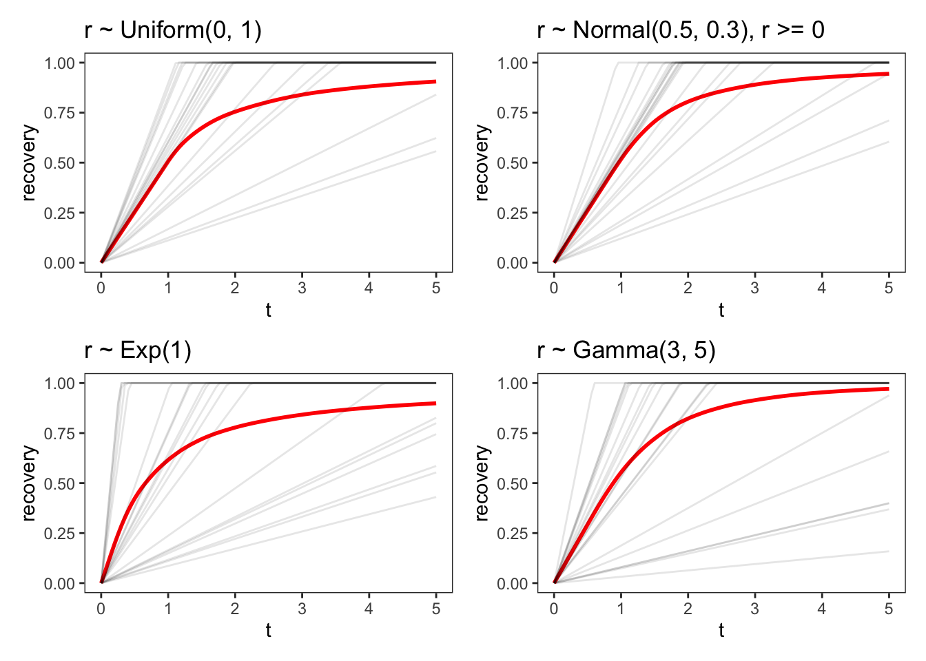
Assume that resource recover linearly over time at a constant rate r until they reach a maximum value of 1. Assume that r is a random variable. Let’s plot the average resource recovery over time under different assumptions about the distribution of r.
Code
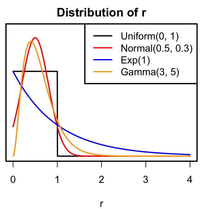
par(mar =c(4, 0.5, 2, 1), lwd =2)curve(dunif(x, 0, 1),from =0, to =4, n =1001, col ="black",xlab ="r", ylab =NA, main ="Distribution of r",ylim =c(0, 1.5), yaxt ="n",)curve( truncnorm::dtruncnorm(x, a =0, mean =0.5, sd =0.3),from =0, to =4, n =1001, col ="red", add =TRUE)curve(dgamma(x, shape =1, scale =1),from =0, to =4, n =1001, col ="blue", add =TRUE)curve(dgamma(x, shape =3, rate =5),from =0, to =4, n =1001, col ="orange", add =TRUE)# add legendlegend("topright",legend =c("Uniform(0, 1)", "Normal(0.5, 0.3)", "Exp(1)", "Gamma(3, 5)"),col =c("black", "red", "blue", "orange"), lty =1)
r is uniformly distributed between 0 and 1.
r is distributed as a truncated normal distribution with mean 0.5 and standard deviation 0.3
r is distributed as an exponential distribution with rate 1
r is distributed as a gamma distribution with shape 3 and rate 5
Red line shows the average recovery over time. Black lines show individual trajectories of a few random samples of r. The full distributions of r are shown in the margin.
Analytical solutions for the average recovery over time
For simplicity, consider the case of recovery starting from 0. Given a continuous distribution of r, \(f(r)\), we can derive the average recovery over time by integrating two separate quantites over all possible values of r. We have to consider two cases:
Resources have not yet reached their maximum value of 1 and are recovering linearly at a rate r. This is the case for \(r < 1/t\)
Resources have reached their maximum value of 1 and are no longer recovering. This is the case for \(r \geq 1/t\)
The average recovery after time t is then given by the following combination of integrals:
\[
R(t) = \int_{0}^{1/t} r \cdot t \cdot f(r) \, dr + \int_{1/t}^{\infty} 1 \cdot f(r) \, dr
\]
Below I give the solution for the exponential and gamma distributions of r.
Exponential distribution
Let’s consider the case where r is distributed as an exponential distribution with rate \(\lambda\). The probability density function of the exponential distribution is given by
where \(\Gamma(a, z)\) is the upper incomplete gamma function, \(\gamma(a, z)\) is the lower incomplete gamma function; and \(P(a, z)\) and \(Q(a, z)\) are the regularized upper and lower incomplete gamma functions, respectively. P and Q are respectively the complimentary cdf and the cdf of the gamma distribution. They can be computed using the pgamma function in R with the lower.tail = FALSE argument for the upper incomplete gamma function and the pgamma function with the lower.tail = TRUE argument for the lower incomplete gamma function.
Compare with exponential recovery
The equations derived above under the assumption of an exponential or gamma distribution of r are obviously not the same as the exponential recovery equation. But is the exponential recovery equation a good approximation of the average recovery over time when r is a random variable following an exponential or gamma distribution?
In this part, I compare the recovery given by the exponential recovery equation with the recovery given by the marginalized linear recovery with r following an exponential distribution or gamma distribution. I will use the analytical solutions derived above to fit the parameters of the exponential and gamma distributions to the exponential recovery equation.
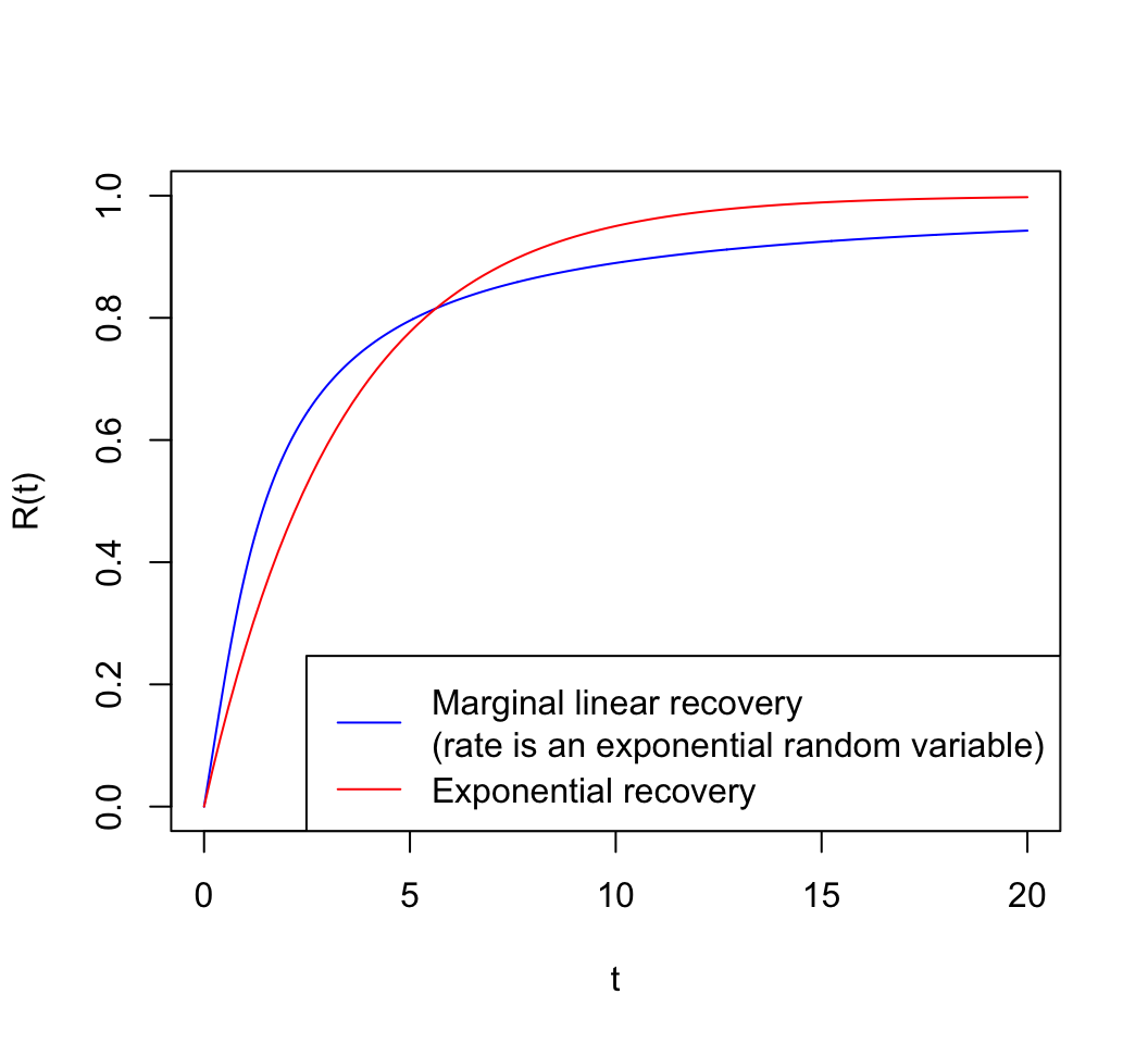
Marginal recovery from an exponential distribution
Set the true recovery rate to 0.3 and fit the rate parameter of the exponential distribution to the exponential recovery equation.
Code
objective_fn <-function(log_lambda, t, target) { pred <-marginal_recovery_exponential(exp(log_lambda), t)sqrt(mean((pred - target)^2))}set.seed(2)true_r <-0.3t <-seq(0, 60, length.out =1000)fit <-optim(1, objective_fn, t = t, target =exp_recovery(true_r, t))lambda <-exp(fit$par)curve(marginal_recovery_exponential(lambda, t),from =0, to =20, n =1001,col ="blue", ylim =c(0, 1), xname ="t", ylab ="R(t)")curve(exp_recovery(true_r, t),col ="red", add =TRUE, xname ="t")legend("bottomright", legend =c("Marginal linear recovery\n(rate is an exponential random variable)", "Exponential recovery"), col =c("blue", "red"), lty =1)
The overall shape is similar, but the approximation is not great.
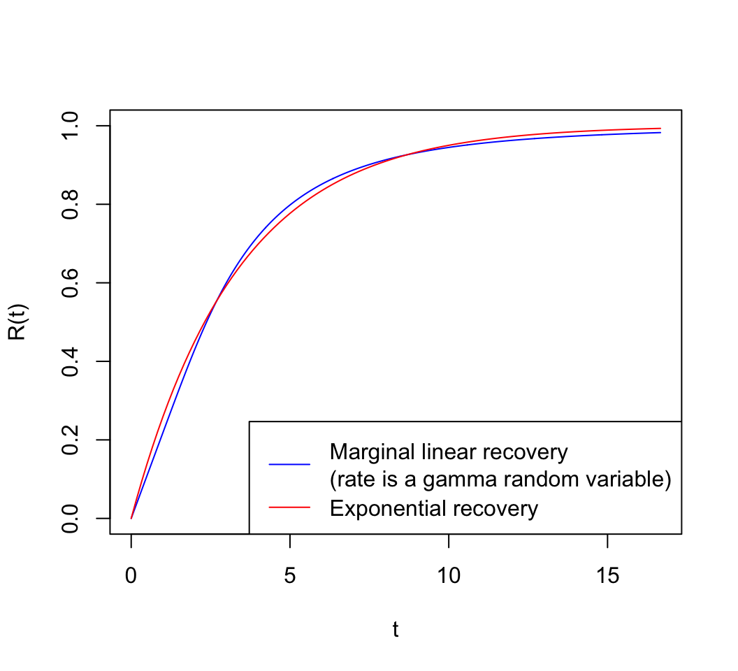
Marginal recovery from a gamma distribution
The approximation when the rate follows a gamma distribution is much better::
Code
objective_fn <-function(pars, t, target) { pred <-marginal_recovery_gamma(exp(pars[1]), exp(pars[2]), t)sqrt(mean((pred - target)^2))}set.seed(2)true_r <-0.30t <-seq(0, 200, length.out =1000)fit <-optim(c(0, 0), objective_fn, t = t, target =exp_recovery(true_r, t))pars <-exp(fit$par)curve(marginal_recovery_gamma(pars[1], pars[2], t),from =0, to =1/ true_r *5, n =1001,col ="blue", ylim =c(0, 1), xname ="t", ylab ="R(t)")curve(exp_recovery(true_r, t),col ="red", add =TRUE, xname ="t")legend("bottomright", legend =c("Marginal linear recovery\n(rate is a gamma random variable)", "Exponential recovery"), col =c("blue", "red"), lty =1)
with an RMSE of 0.005. The fit is basically the same for all values of r.
Summary
The exponential recovery equation is a good approximation of the average recovery over time when the rate of recovery is a random variable following a gamma distribution. The approximation is not as good when the rate of recovery is a random variable following an exponential distribution.
Conversion of parameters
Optional
The section below is not directly relevant to our project, but I found the results quite fascinating. Feel free to skip it if you are not interested in the relationship between the parameters of the gamma distribution and the true recovery rate.
When the rate of recovery is a random variable following a gamma distribution, this is approximated well by the exponential recovery equation. The gamma distribution has two parameters: the shape parameter \(\alpha\) and the rate parameter \(\lambda\), while the exponential recovery equation has only one parameter: the rate of recovery r. How do the parameters of the gamma distribution relate to the recovery rate in exponential recovery equation?
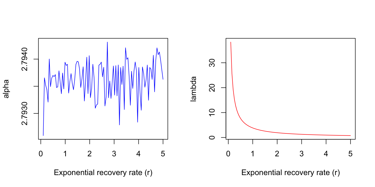
I will simulate the recovery over time for different values of the true recovery rate r in the range [0.1, 5]. Then I will fit to this the marginal recovery predicted by a linear recovery process where the rate follows a gamma distribution. I will then explore the relationship between the parameters of the gamma distribution and the true recovery rate.
Code
t <-seq(0, 200, length.out =10000)get_pars <-function(true_r, t) { objective_fn <-function(pars, t, target) { pred <-marginal_recovery_gamma(exp(pars[1]), exp(pars[2]), t)sqrt(mean((pred - target)^2)) } fit <-optim(c(0, 0), objective_fn, t = t, target =exp_recovery(true_r, t)) pars <-exp(fit$par) pars}true_r <-seq(0.1, 5, length.out =100)pars <-run_or_load(sapply(true_r, get_pars, t = t), "output/gamma_recovery_pars.rds")par(mfrow =c(1, 2))plot(true_r, pars[1, ], type ="l", col ="blue", xlab ="Exponential recovery rate (r)", ylab ="alpha")plot(true_r, pars[2, ], type ="l", col ="red", xlab ="Exponential recovery rate (r)", ylab ="lambda")
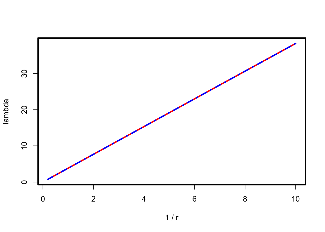
I did not expect this. The shape parameter \(\alpha\) is fixed at 2.7937 and only the rate \(\lambda\) changes. Turns out that lambda is linearly related to 1/r (red line is the “data” and blue line is the fitted line from a linear regression):
Code
par(mfrow =c(1, 1), lwd =3)plot(1/ true_r, pars[2, ], type ="l", col ="red", xlab ="1 / r", ylab ="lambda")lines(pars[2, ] ~I(1/ true_r), col ="blue", lty =4)
with the following relationship:
\[
\lambda \approxeq 3.831 \,r^{-1}
\]
Summary
An exponential recovery processes with rate \(r\) can be approximated well by a linear recovery process where the rate of recovery is a random variable which follows a gamma distribution with shape parameter \(\alpha =\) 2.794 and rate parameter \(\lambda = 3.831 \,r^{-1}\). That is, modeling resource recovery with the following two equations is almost equivalent:
---title: "Linear recovery as a random variable"format: htmlauthor: "Ven Popov"date: 05/27/2024date-modified: 05/28/2024---```{r init, include = FALSE}#| message: falselibrary(ggplot2)library(dplyr)library(targets)library(patchwork)tar_source()```## OverviewIn the simulations we have considered two different equations for the recovery of resources over time:#### Linear recoveryResources recover linearly over time at a constant rate `r` until they reach a maximum value of 1:$$R_{new} = \min(1, R + r \cdot t)$$where $R$ is the resource level before recovery, $t$ is the recovery duration, and $r$ is the recovery rate.#### Exponential recoveryAlternatively, resources could recover non-linearly over time at a rate that depends on the current resource level:$$R_{new} = R + (1 - R) \cdot (1 - e^{-r t}) = 1 - (1 - R)e^{-r t}$$which can be simplified in the case of recovery starting from 0 to$$R(t) = 1 - e^{-r t}$$Klaus and I discussed the possibility that the recovery is linear, but the rate of recovery `r` is a random variable that varies over trials and individuals. Similarly to the evidence accumulation rate in the linear balistic accumulator models, at the aggregate level the recovery rate might be better modeled with the exponential recovery equation, even if the individual recovery is linear. In this notebook, I explore this idea further and derive analytical solutions for the average recovery over time under different assumptions about the distribution of `r`.## Linear recovery with a random variable rateAssume that resource recover linearly over time at a constant rate `r` until they reach a maximum value of 1. Assume that `r` is a random variable. Let's plot the average resource recovery over time under different assumptions about the distribution of `r`.```{r}#| fig-column: margin#| results: hold#| fig-width: 3.5#| fig-height: 3.5par(mar =c(4, 0.5, 2, 1), lwd =2)curve(dunif(x, 0, 1),from =0, to =4, n =1001, col ="black",xlab ="r", ylab =NA, main ="Distribution of r",ylim =c(0, 1.5), yaxt ="n",)curve( truncnorm::dtruncnorm(x, a =0, mean =0.5, sd =0.3),from =0, to =4, n =1001, col ="red", add =TRUE)curve(dgamma(x, shape =1, scale =1),from =0, to =4, n =1001, col ="blue", add =TRUE)curve(dgamma(x, shape =3, rate =5),from =0, to =4, n =1001, col ="orange", add =TRUE)# add legendlegend("topright",legend =c("Uniform(0, 1)", "Normal(0.5, 0.3)", "Exp(1)", "Gamma(3, 5)"),col =c("black", "red", "blue", "orange"), lty =1)```1. `r` is uniformly distributed between 0 and 1.2. `r` is distributed as a truncated normal distribution with mean 0.5 and standard deviation 0.33. `r` is distributed as an exponential distribution with rate 14. `r` is distributed as a gamma distribution with shape 3 and rate 5Red line shows the average recovery over time. Black lines show individual trajectories of a few random samples of `r`. The full distributions of `r` are shown in the margin.```{r}set.seed(3)n <-1000r_unif <-runif(n, 0, 1)r_truncnorm <- truncnorm::rtruncnorm(n, a =0, mean =0.5, sd =0.3)r_exp <-rgamma(n, shape =1, scale =1)r_gamma <-rgamma(n, shape =3, rate =5)t <-seq(0, 5, length.out =100)plot_linear_rv_recovery(r_unif, t, title ="r ~ Uniform(0, 1)") +plot_linear_rv_recovery(r_truncnorm, t, title ="r ~ Normal(0.5, 0.3), r >= 0") +plot_linear_rv_recovery(r_exp, t, "r ~ Exp(1)") +plot_linear_rv_recovery(r_gamma, t, "r ~ Gamma(3, 5)")```## Analytical solutions for the average recovery over timeFor simplicity, consider the case of recovery starting from 0. Given a continuous distribution of `r`, $f(r)$, we can derive the average recovery over time by integrating two separate quantites over all possible values of `r`. We have to consider two cases:1. Resources have not yet reached their maximum value of 1 and are recovering linearly at a rate `r`. This is the case for $r < 1/t$2. Resources have reached their maximum value of 1 and are no longer recovering. This is the case for $r \geq 1/t$The average recovery after time `t` is then given by the following combination of integrals:$$R(t) = \int_{0}^{1/t} r \cdot t \cdot f(r) \, dr + \int_{1/t}^{\infty} 1 \cdot f(r) \, dr $$Below I give the solution for the exponential and gamma distributions of `r`.### Exponential distributionLet's consider the case where `r` is distributed as an exponential distribution with rate $\lambda$. The probability density function of the exponential distribution is given by$$f(r) = \lambda e^{-\lambda r}$$The average recovery over time is then given by\begin{aligned}R(t) &= \int_{0}^{1/t} r \cdot t \cdot \lambda e^{-\lambda r} \, dr + \int_{1/t}^{\infty} 1 \cdot \lambda e^{-\lambda r} \, dr \\&= \left[ -\frac{t e^{\lambda (-r)} (\lambda r+1)}{\lambda } \right]_{0}^{1/t} + \left[ -e^{-\lambda r} \right]_{1/t}^{\infty} \\&= \frac{t-e^{-\lambda / t} (\lambda +t)}{\lambda } + e^{-\lambda / t} \\&= \frac{t}{\lambda} (1 - e^{-\lambda/t})\end{aligned}### Gamma distributionThe probability density function of the gamma distribution is given by$$f(r) = \frac{\lambda^{\alpha} r^{\alpha - 1} e^{-\lambda r}}{\Gamma(\alpha)}$$where $\alpha$ is the shape parameter and $\lambda$ is the rate parameter. The average recovery over time is then given by$$\begin{aligned}R(t) &= \int_{0}^{1/t} r \cdot t \cdot \frac{\lambda^{\alpha} r^{\alpha - 1} e^{-\lambda r}}{\Gamma(\alpha)} \, dr + \int_{1/t}^{\infty} 1 \cdot \frac{\lambda^{\alpha} r^{\alpha - 1} e^{-\lambda r}}{\Gamma(\alpha)} \, dr \\&= \frac{\lambda^{\alpha}}{\Gamma(\alpha)} \left( t \int_{0}^{1/t} r^{\alpha} e^{-\lambda r} \, dr + \int_{1/t}^{\infty} r^{\alpha - 1} e^{-\lambda r} \, dr \right) \\\end{aligned}$$which after some transformations can be written as$$\begin{aligned}R(t) &= \frac{\Gamma \left(\alpha ,\frac{\lambda }{t}\right)}{\Gamma (\alpha )}+\frac{\alpha t}{\lambda}\frac{\gamma \left(\alpha +1,\frac{\lambda }{t}\right)}{\Gamma (\alpha +1)} \\&= P(\alpha, \lambda / t) + \frac{\alpha t}{\lambda} Q(\alpha + 1, \lambda / t)\end{aligned}$$where $\Gamma(a, z)$ is the [upper incomplete gamma function](https://mathworld.wolfram.com/IncompleteGammaFunction.html), $\gamma(a, z)$ is the lower incomplete gamma function; and $P(a, z)$ and $Q(a, z)$ are the regularized upper and lower incomplete gamma functions, respectively. P and Q are respectively the complimentary cdf and the cdf of the gamma distribution. They can be computed using the `pgamma` function in R with the `lower.tail = FALSE` argument for the upper incomplete gamma function and the `pgamma` function with the `lower.tail = TRUE` argument for the lower incomplete gamma function.## Compare with exponential recoveryThe equations derived above under the assumption of an exponential or gamma distribution of `r` are obviously not the same as the exponential recovery equation. But is the exponential recovery equation a good approximation of the average recovery over time when `r` is a random variable following an exponential or gamma distribution?In this part, I compare the recovery given by the exponential recovery equation with the recovery given by the marginalized linear recovery with `r` following an exponential distribution or gamma distribution. I will use the analytical solutions derived above to fit the parameters of the exponential and gamma distributions to the exponential recovery equation.Let's define our functions:```{r}#| code-fold: falseexp_recovery <-function(r, t) {1-exp(-r * t)}marginal_recovery_exponential <-function(lambda, t) { t/lambda * (1-exp(-lambda/t))}marginal_recovery_gamma <-function(alpha, lambda, t) { P <-pgamma(lambda / t, shape = alpha, lower.tail =FALSE) R <-pgamma(lambda / t, shape = alpha +1) P + alpha * t / lambda * R}```### Marginal recovery from an exponential distributionSet the true recovery rate to 0.3 and fit the rate parameter of the exponential distribution to the exponential recovery equation.```{r}#| warning: false#| message: false#| fig-width: 5.5#| fig-height: 5objective_fn <-function(log_lambda, t, target) { pred <-marginal_recovery_exponential(exp(log_lambda), t)sqrt(mean((pred - target)^2))}set.seed(2)true_r <-0.3t <-seq(0, 60, length.out =1000)fit <-optim(1, objective_fn, t = t, target =exp_recovery(true_r, t))lambda <-exp(fit$par)curve(marginal_recovery_exponential(lambda, t),from =0, to =20, n =1001,col ="blue", ylim =c(0, 1), xname ="t", ylab ="R(t)")curve(exp_recovery(true_r, t),col ="red", add =TRUE, xname ="t")legend("bottomright", legend =c("Marginal linear recovery\n(rate is an exponential random variable)", "Exponential recovery"), col =c("blue", "red"), lty =1)```The overall shape is similar, but the approximation is not great. ### Marginal recovery from a gamma distributionThe approximation when the rate follows a gamma distribution is much better::```{r}#| warning: false#| message: false#| fig-width: 5.5#| fig-height: 5objective_fn <-function(pars, t, target) { pred <-marginal_recovery_gamma(exp(pars[1]), exp(pars[2]), t)sqrt(mean((pred - target)^2))}set.seed(2)true_r <-0.30t <-seq(0, 200, length.out =1000)fit <-optim(c(0, 0), objective_fn, t = t, target =exp_recovery(true_r, t))pars <-exp(fit$par)curve(marginal_recovery_gamma(pars[1], pars[2], t),from =0, to =1/ true_r *5, n =1001,col ="blue", ylim =c(0, 1), xname ="t", ylab ="R(t)")curve(exp_recovery(true_r, t),col ="red", add =TRUE, xname ="t")legend("bottomright", legend =c("Marginal linear recovery\n(rate is a gamma random variable)", "Exponential recovery"), col =c("blue", "red"), lty =1)```with an RMSE of `r round(fit$value, 4)`. The fit is basically the same for all values of `r`. ::: {.callout-important}## SummaryThe exponential recovery equation is a good approximation of the average recovery over time when the rate of recovery is a random variable following a gamma distribution. The approximation is not as good when the rate of recovery is a random variable following an exponential distribution.:::## Conversion of parameters::: {.callout-note}## OptionalThe section below is not directly relevant to our project, but I found the results quite fascinating. Feel free to skip it if you are not interested in the relationship between the parameters of the gamma distribution and the true recovery rate.:::When the rate of recovery is a random variable following a gamma distribution, this is approximated well by the exponential recovery equation. The gamma distribution has two parameters: the shape parameter $\alpha$ and the rate parameter $\lambda$, while the exponential recovery equation has only one parameter: the rate of recovery `r`. How do the parameters of the gamma distribution relate to the recovery rate in exponential recovery equation?I will simulate the recovery over time for different values of the true recovery rate `r` in the range [0.1, 5]. Then I will fit to this the marginal recovery predicted by a linear recovery process where the rate follows a gamma distribution. I will then explore the relationship between the parameters of the gamma distribution and the true recovery rate.```{r}#| fig-width: 8#| fig-height: 4t <-seq(0, 200, length.out =10000)get_pars <-function(true_r, t) { objective_fn <-function(pars, t, target) { pred <-marginal_recovery_gamma(exp(pars[1]), exp(pars[2]), t)sqrt(mean((pred - target)^2)) } fit <-optim(c(0, 0), objective_fn, t = t, target =exp_recovery(true_r, t)) pars <-exp(fit$par) pars}true_r <-seq(0.1, 5, length.out =100)pars <-run_or_load(sapply(true_r, get_pars, t = t), "output/gamma_recovery_pars.rds")par(mfrow =c(1, 2))plot(true_r, pars[1, ], type ="l", col ="blue", xlab ="Exponential recovery rate (r)", ylab ="alpha")plot(true_r, pars[2, ], type ="l", col ="red", xlab ="Exponential recovery rate (r)", ylab ="lambda")```I did not expect this. The shape parameter $\alpha$ is fixed at `r round(median(pars[1, ]),4)` and only the rate $\lambda$ changes. Turns out that lambda is linearly related to 1/r (red line is the "data" and blue line is the fitted line from a linear regression):```{r}par(mfrow =c(1, 1), lwd =3)plot(1/ true_r, pars[2, ], type ="l", col ="red", xlab ="1 / r", ylab ="lambda")lines(pars[2, ] ~I(1/ true_r), col ="blue", lty =4)```with the following relationship:$$\lambda \approxeq 3.831 \,r^{-1}$$## SummaryAn exponential recovery processes with rate $r$ can be approximated well by a linear recovery process where the rate of recovery is a random variable which follows a gamma distribution with shape parameter $\alpha =$ `r round(median(pars[1, ]),3)` and rate parameter $\lambda = 3.831 \,r^{-1}$. That is, modeling resource recovery with the following two equations is almost equivalent:$$R(t) = 1 - e^{-r t}$$and$$R(t) = min(1, r_{linear}t) \\$$$$r_{linear} \sim \text{Gamma}(2.794, 3.831 \cdot r^{-1})$$