Code
library(tidyverse)
library(targets)
library(GGally)
library(kableExtra)
# load "R/*" scripts and saved R objects from the targets pi
tar_source()
tar_load(c(exp1_data_agg_enc, exp2_data_agg_enc, fits3))library(tidyverse)
library(targets)
library(GGally)
library(kableExtra)
# load "R/*" scripts and saved R objects from the targets pi
tar_source()
tar_load(c(exp1_data_agg_enc, exp2_data_agg_enc, fits3))Here I employ the same model as in Model 1 with one difference. In the previous model, the encoding time was not included. It assumed that during encoding of the triplets (0.9 seconds), nothing happened, and recovery of resources only started after the encoding was completed. In Popov & Reder (2020), we assumed that depletion happens instantaneously, and recovery continuous thoughout the encoding and inter-stimulus interval.
So here we just add the 0.9 seconds of encoding time to the ISI. For example, this is coded in the ISI column:
exp1_data_agg_enc |>
  kbl() |>
kable_styling()| chunk | gap | itemtype | n_total | n_correct | p_correct | ISI | item_in_ltm |
|---|---|---|---|---|---|---|---|
| known | 500 | SP1-3 | 1855 | 1715 | 0.9245283 | 1.4 | TRUE |
| known | 500 | SP4-6 | 1858 | 1368 | 0.7362756 | 1.4 | FALSE |
| known | 500 | SP7-9 | 1851 | 943 | 0.5094543 | 1.4 | FALSE |
| known | 3000 | SP1-3 | 1859 | 1721 | 0.9257665 | 3.9 | TRUE |
| known | 3000 | SP4-6 | 1858 | 1443 | 0.7766416 | 1.4 | FALSE |
| known | 3000 | SP7-9 | 1856 | 1032 | 0.5560345 | 1.4 | FALSE |
| random | 500 | SP1-3 | 1853 | 1495 | 0.8067998 | 1.4 | FALSE |
| random | 500 | SP4-6 | 1856 | 1177 | 0.6341595 | 1.4 | FALSE |
| random | 500 | SP7-9 | 1855 | 727 | 0.3919137 | 1.4 | FALSE |
| random | 3000 | SP1-3 | 1856 | 1553 | 0.8367457 | 3.9 | FALSE |
| random | 3000 | SP4-6 | 1858 | 1287 | 0.6926803 | 1.4 | FALSE |
| random | 3000 | SP7-9 | 1856 | 838 | 0.4515086 | 1.4 | FALSE |
# calculate deviance and predictions
fits3 <- fits3 |>
  mutate(
    deviance = pmap_dbl(
      list(fit, data, exclude_sp1),
      ~ overall_deviance(params = `..1`$par, data = `..2`, exclude_sp1 = `..3`)
    ),
    pred = map2(fit, data, ~ predict(.x, .y, group_by = c("chunk", "gap")))
  )
(just like in Model 1, I fit the data by either excluding the first serial position or not, and including priors on the gain and rate parameters or not).
These are the best fitting parameters for each experiment, prior scenario, and whether the first serial position was excluded or not:
final3 <- fits3 |>
  filter(convergence == 0) |>
  group_by(exp, priors_scenario, exclude_sp1) |>
  arrange(deviance) |>
  slice(1) |>
  arrange(desc(exclude_sp1), exp, priors_scenario) |>
  mutate(
    deviance = round(deviance, 1),
    priors_scenario = case_when(
      priors_scenario == "none" ~ "None",
      priors_scenario == "gain" ~ "Gain ~ N(25, 0.1)",
      priors_scenario == "rate" ~ "Rate ~ N(0.1, 0.01)"
    )
  )

final3 |>
  select(exp, priors_scenario, exclude_sp1, prop:gain, deviance) |>
  mutate_all(round, 3) |>
  kbl() |>
kable_styling()| exp | priors_scenario | exclude_sp1 | prop | prop_ltm | rate | tau | gain | deviance |
|---|---|---|---|---|---|---|---|---|
| 1 | Gain ~ N(25, 0.1) | TRUE | 0.231 | 0.617 | 0.018 | 0.162 | 25.001 | 33.1 |
| 1 | None | TRUE | 0.110 | 0.606 | 0.009 | 0.094 | 99.996 | 31.9 |
| 1 | Rate ~ N(0.1, 0.01) | TRUE | 0.435 | 0.646 | 0.043 | 0.222 | 8.364 | 42.4 |
| 2 | Gain ~ N(25, 0.1) | TRUE | 0.211 | 0.834 | 0.013 | 0.153 | 25.000 | 40.7 |
| 2 | None | TRUE | 0.106 | 0.826 | 0.006 | 0.091 | 91.036 | 40.5 |
| 2 | Rate ~ N(0.1, 0.01) | TRUE | 0.473 | 0.855 | 0.030 | 0.212 | 6.286 | 46.5 |
| 1 | Gain ~ N(25, 0.1) | FALSE | 0.239 | 0.660 | 0.016 | 0.163 | 24.998 | 145.4 |
| 1 | None | FALSE | 0.302 | 0.658 | 0.020 | 0.184 | 16.186 | 144.9 |
| 1 | Rate ~ N(0.1, 0.01) | FALSE | 0.472 | 0.673 | 0.044 | 0.220 | 7.604 | 152.2 |
| 2 | Gain ~ N(25, 0.1) | FALSE | 0.222 | 0.879 | 0.011 | 0.155 | 24.998 | 113.3 |
| 2 | None | FALSE | 0.379 | 0.868 | 0.019 | 0.198 | 9.421 | 109.7 |
| 2 | Rate ~ N(0.1, 0.01) | FALSE | 0.497 | 0.865 | 0.030 | 0.209 | 5.950 | 113.4 |
for comparison, here are the results of Model 1
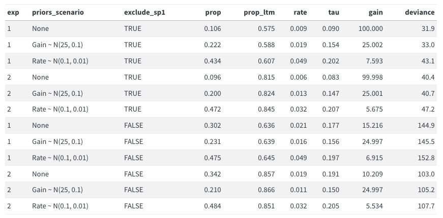
Doesn’t make much of a difference. Do not pursue further.