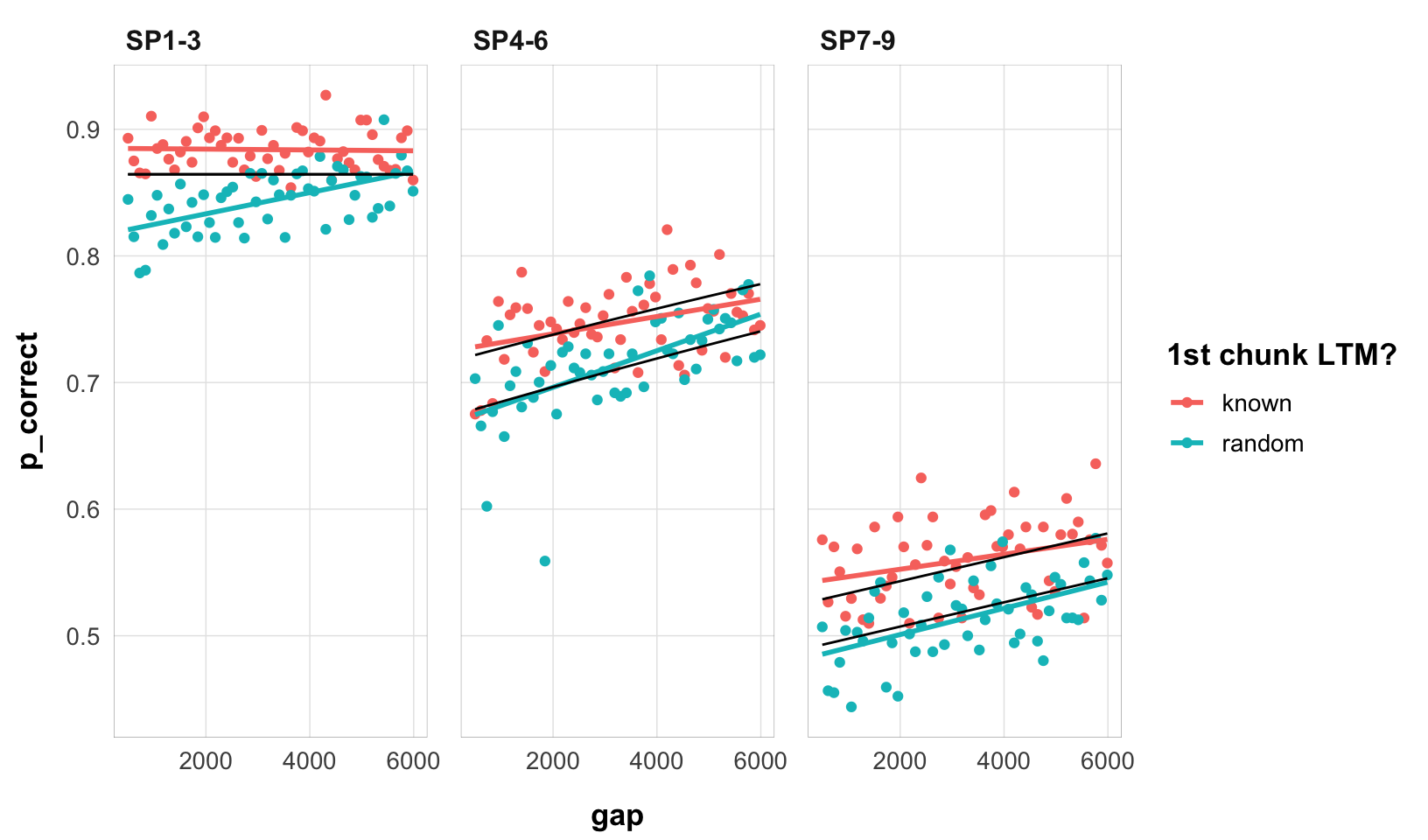
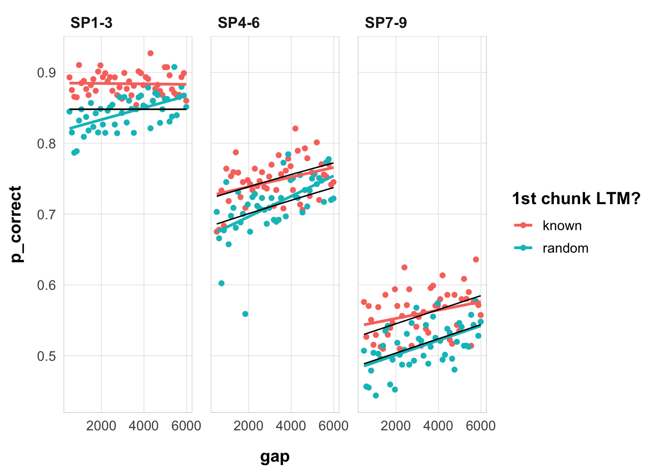
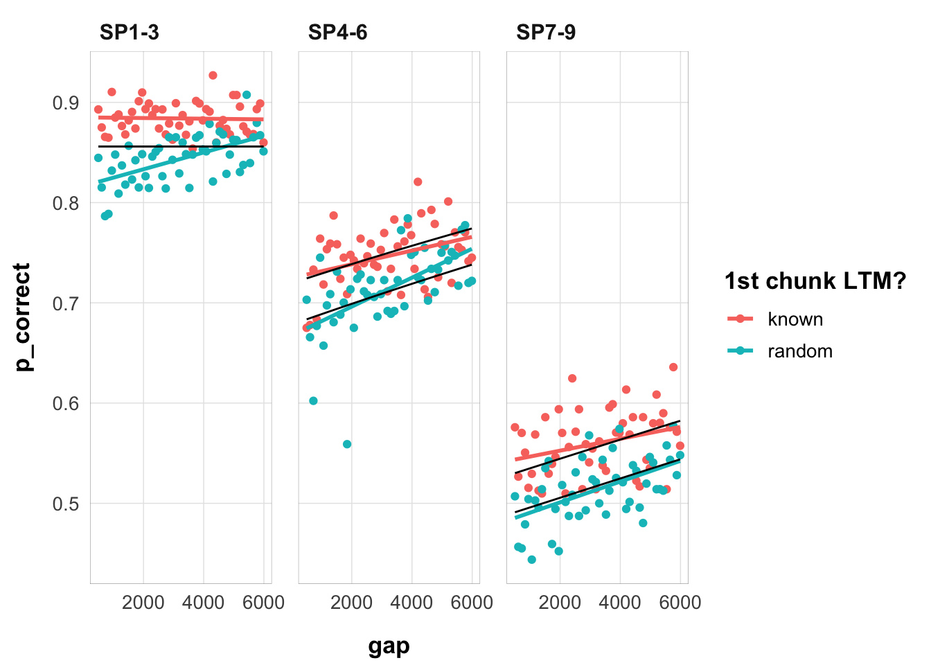
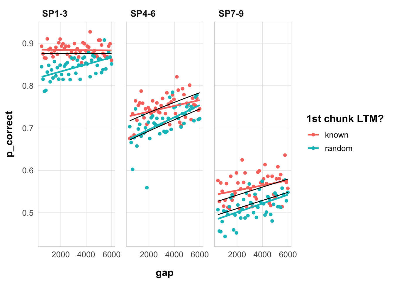
Free time & chunking modeling
  • Versions
    • Latest
    • v0.1
  • Source Code
  • Report a Bug
  1. Notebooks
  2. Model 1: Original model
  3. Experiment 3
  • Version 0.1
  •  
  • About
  • Development notes
    • Notes
    • 2024-05-16 Meeting Notes
    • Extra primacy parameter
  • Notebooks
    • Data
      • View the data structure
      • Exploratory data analysis
      • Subject-level data
    • Model 1: Original model
      • Main results
      • Parameter identifiability
      • Sensitivity to tau
      • Experiment 3
      • Exploring model predictions
    • Model 2: Include encoding time
      • Main results
    • Model 3: Non-linear recovery
      • Explore model predictions
      • Basic fits
      • Bootstrapping data and fits for parameter uncertainty estimation
      • Extra primacy parameter
      • Linear recovery as a random variable
  • Function reference
    • Aggregate Data
    • Perform bootstrapped estimation
    • Calculate the deviance of a model
    • Get data object from a file
    • Generate a bootstrapped dataset
    • get_data function
    • Inverse Logit Transformation
    • Logit Transformation
    • Calculate the overall deviance
    • Plot Bootstrap Results
    • Plot Linear RV Recovery
    • Preprocesses the data
    • Execute an expression and save the result to a file or load the result from a file if it already exists.
    • Serial Recall Model

On this page

  • Basic fit
    • Trying priors of the gain parameter
    • Trying priors of the rate parameter
  • Summary
  1. Notebooks
  2. Model 1: Original model
  3. Experiment 3

Experiment 3

  • Show All Code
  • Hide All Code

  • View Source
Code
library(tidyverse)
library(targets)
tar_source()
tar_load(c(exp3_data_agg))
tar_load(fits1)

fits1_e3 <- fits1 |>
  filter(exp == 3) |>
  mutate(
    deviance = pmap_dbl(
      list(fit, data, exclude_sp1),
      ~ overall_deviance(params = `..1`$par, data = `..2`, exclude_sp1 = `..3`)
    ),
    pred = map2(fit, data, ~ predict(.x, .y, group_by = c("chunk", "gap")))
  )

Basic fit

Fit starting from the parameters reported in the draft for Experiment 1:

Code
est <- run_or_load(
  estimate_model(
    start = paper_params(),
    data = exp3_data_agg,
    two_step = TRUE,
    exclude_sp1 = TRUE,
    simplify = TRUE,
    prior = list(
      rate = list(mean = 0.05, sd = 0.01)
    )
  ),
  file = "output/exp3_basic_fit.rds"
)

est
# A tibble: 1 × 8
   prop prop_ltm   rate   tau  gain deviance convergence fit       
  <dbl>    <dbl>  <dbl> <dbl> <dbl>    <dbl>       <int> <list>    
1 0.296    0.819 0.0143 0.153  12.9     769.           0 <srl_rcl_>
Code
exp3_data_agg$pred <- predict(est$fit[[1]], data = exp3_data_agg, group_by = c("chunk", "gap"))

exp3_data_agg |>
  ggplot(aes(gap, p_correct, color = chunk, group = chunk)) +
  geom_point() +
  stat_smooth(method = "lm", se = FALSE) +
  geom_line(aes(y = pred), color = "black") +
  scale_color_discrete("1st chunk LTM?") +
  facet_wrap(~itemtype) +
  theme_pub()
`geom_smooth()` using formula = 'y ~ x'

These are the best fitting parameters when running with 100 different starting points:

Code
fits1_e3 |>
  filter(exclude_sp1 == TRUE, priors_scenario == "none") |>
  arrange(deviance) |>
  select(prop:deviance) |>
  head(15) |>
  kableExtra::kable()
prop prop_ltm rate tau gain deviance
0.1176852 0.8038622 0.0056074 0.0928974 69.325675 764.8021
0.1171605 0.8039528 0.0055792 0.0925837 69.905273 764.8022
0.1158791 0.8034533 0.0055264 0.0918260 71.369326 764.8022
0.1171228 0.8034459 0.0055762 0.0925632 69.947438 764.8023
0.1223134 0.8039849 0.0058120 0.0955887 64.418454 764.8032
0.1184461 0.8040876 0.0056514 0.0933540 68.472023 764.8049
0.1169663 0.8037114 0.0055752 0.0924832 70.135163 764.8066
0.1255808 0.8051079 0.0060152 0.0974679 61.297036 764.8067
0.1357685 0.8044079 0.0064193 0.1030411 52.924650 764.8160
0.1169577 0.8037673 0.0055755 0.0924814 70.102525 764.8164
0.1516215 0.8060898 0.0071830 0.1111224 43.004528 764.8409
0.5709167 0.4530002 0.2213147 0.2424797 3.249835 848.5274
0.5710025 0.4530985 0.2213565 0.2424506 3.248783 848.5274
0.5711107 0.4530694 0.2213929 0.2424626 3.247816 848.5274
0.5706589 0.4531750 0.2211694 0.2424859 3.252406 848.5275

The fits require very slow rate again. Here’s the plot of the best fitting parameters:

Code
fits1_e3 |>
  filter(exp == 3, exclude_sp1 == TRUE, priors_scenario == "none") |>
  arrange(deviance) |> 
  slice(1) |>
  select(data, pred) |>
  unnest(cols = everything()) |>
  ggplot(aes(gap, p_correct, color = chunk, group = chunk)) +
  geom_point() +
  stat_smooth(method = "lm", se = FALSE) +
  geom_line(aes(y = pred), color = "black") +
  scale_color_discrete("1st chunk LTM?") +
  facet_wrap(~itemtype) +
  theme_pub()
`geom_smooth()` using formula = 'y ~ x'

Trying priors of the gain parameter

Like for Experiment 1, restrict the gain to be ~ 25

Code
fits1_e3 |>
  filter(priors_scenario == "gain", exclude_sp1 == TRUE, convergence == 0) |>
  select(prop:convergence) |>
  arrange(deviance) |>
  mutate_all(round, 3) |>
  print(n = 10)
# A tibble: 100 × 7
    prop prop_ltm  rate   tau  gain deviance convergence
   <dbl>    <dbl> <dbl> <dbl> <dbl>    <dbl>       <dbl>
 1 0.204    0.811  0.01 0.132  25.0     765.           0
 2 0.204    0.81   0.01 0.132  25.0     765.           0
 3 0.204    0.811  0.01 0.132  25       765.           0
 4 0.204    0.811  0.01 0.132  25.0     765.           0
 5 0.204    0.811  0.01 0.132  25       765.           0
 6 0.204    0.81   0.01 0.132  25       765.           0
 7 0.204    0.811  0.01 0.132  25.0     765.           0
 8 0.204    0.811  0.01 0.132  25       765.           0
 9 0.204    0.81   0.01 0.132  25.0     765.           0
10 0.204    0.81   0.01 0.132  25.0     765.           0
# ℹ 90 more rows

plot of the best fitting parameters:

Code
fits1_e3 |>
  filter(priors_scenario == "gain", exclude_sp1 == TRUE, convergence == 0) |>
  arrange(deviance) |> 
  slice(1) |>
  select(data, pred) |>
  unnest(cols = everything()) |>
  ggplot(aes(gap, p_correct, color = chunk, group = chunk)) +
  geom_point() +
  stat_smooth(method = "lm", se = FALSE) +
  geom_line(aes(y = pred), color = "black") +
  scale_color_discrete("1st chunk LTM?") +
  facet_wrap(~itemtype) +
  theme_pub()
`geom_smooth()` using formula = 'y ~ x'

Trying priors of the rate parameter

Like for Experiment 1, rate parameter prior ~ Normal(0.1, 0.01)

Code
fits1_e3 |>
  filter(priors_scenario == "rate", exclude_sp1 == TRUE, convergence == 0) |>
  select(prop:convergence) |>
  arrange(deviance) |>
  mutate_all(round, 3) |>
  print(n = 10)
# A tibble: 98 × 7
    prop prop_ltm  rate   tau  gain deviance convergence
   <dbl>    <dbl> <dbl> <dbl> <dbl>    <dbl>       <dbl>
 1 0.404    0.831 0.021 0.153  7.74     770.           0
 2 0.407    0.832 0.021 0.152  7.65     770.           0
 3 0.408    0.832 0.021 0.152  7.63     770.           0
 4 0.408    0.832 0.021 0.152  7.64     770.           0
 5 0.408    0.832 0.021 0.152  7.62     770.           0
 6 0.408    0.832 0.021 0.152  7.62     770.           0
 7 0.408    0.832 0.021 0.152  7.62     770.           0
 8 0.408    0.832 0.021 0.152  7.62     770.           0
 9 0.408    0.832 0.021 0.152  7.62     770.           0
10 0.409    0.832 0.021 0.152  7.61     770.           0
# ℹ 88 more rows

plot of the best fitting parameters:

Code
fits1_e3 |>
  filter(priors_scenario == "rate", exclude_sp1 == TRUE, convergence == 0) |>
  arrange(deviance) |> 
  slice(1) |>
  select(data, pred) |>
  unnest(cols = everything()) |>
  ggplot(aes(gap, p_correct, color = chunk, group = chunk)) +
  geom_point() +
  stat_smooth(method = "lm", se = FALSE) +
  geom_line(aes(y = pred), color = "black") +
  scale_color_discrete("1st chunk LTM?") +
  facet_wrap(~itemtype) +
  theme_pub()
`geom_smooth()` using formula = 'y ~ x'

Summary

The linear recovery model cannot fit the interaction present in the data. As discussed elsewhere, this is because in order to capture the primacy effect and the global proactive benefit of free time, it needs low depletion and low recovery rates.

Back to top
Sensitivity to tau
Exploring model predictions
Source Code
---
title: "Experiment 3"
format: html
---

```{r}
#| label: init
#| message: false
library(tidyverse)
library(targets)
tar_source()
tar_load(c(exp3_data_agg))
tar_load(fits1)

fits1_e3 <- fits1 |>
  filter(exp == 3) |>
  mutate(
    deviance = pmap_dbl(
      list(fit, data, exclude_sp1),
      ~ overall_deviance(params = `..1`$par, data = `..2`, exclude_sp1 = `..3`)
    ),
    pred = map2(fit, data, ~ predict(.x, .y, group_by = c("chunk", "gap")))
  )
```

## Basic fit

Fit starting from the parameters reported in the draft for Experiment 1:

```{r}
est <- run_or_load(
  estimate_model(
    start = paper_params(),
    data = exp3_data_agg,
    two_step = TRUE,
    exclude_sp1 = TRUE,
    simplify = TRUE,
    prior = list(
      rate = list(mean = 0.05, sd = 0.01)
    )
  ),
  file = "output/exp3_basic_fit.rds"
)

est
```

```{r}
#| label: exp3_performance
#| fig-width: 8.5
#| fig-height: 5
exp3_data_agg$pred <- predict(est$fit[[1]], data = exp3_data_agg, group_by = c("chunk", "gap"))

exp3_data_agg |>
  ggplot(aes(gap, p_correct, color = chunk, group = chunk)) +
  geom_point() +
  stat_smooth(method = "lm", se = FALSE) +
  geom_line(aes(y = pred), color = "black") +
  scale_color_discrete("1st chunk LTM?") +
  facet_wrap(~itemtype) +
  theme_pub()

```

These are the best fitting parameters when running with 100 different starting points: 

```{r}
fits1_e3 |>
  filter(exclude_sp1 == TRUE, priors_scenario == "none") |>
  arrange(deviance) |>
  select(prop:deviance) |>
  head(15) |>
  kableExtra::kable()
```

The fits require very slow rate again. Here's the plot of the best fitting parameters:

```{r}
fits1_e3 |>
  filter(exp == 3, exclude_sp1 == TRUE, priors_scenario == "none") |>
  arrange(deviance) |> 
  slice(1) |>
  select(data, pred) |>
  unnest(cols = everything()) |>
  ggplot(aes(gap, p_correct, color = chunk, group = chunk)) +
  geom_point() +
  stat_smooth(method = "lm", se = FALSE) +
  geom_line(aes(y = pred), color = "black") +
  scale_color_discrete("1st chunk LTM?") +
  facet_wrap(~itemtype) +
  theme_pub()
```

### Trying priors of the gain parameter

Like for Experiment 1, restrict the gain to be ~ 25

```{r}
fits1_e3 |>
  filter(priors_scenario == "gain", exclude_sp1 == TRUE, convergence == 0) |>
  select(prop:convergence) |>
  arrange(deviance) |>
  mutate_all(round, 3) |>
  print(n = 10)
```


plot of the best fitting parameters:

```{r}
fits1_e3 |>
  filter(priors_scenario == "gain", exclude_sp1 == TRUE, convergence == 0) |>
  arrange(deviance) |> 
  slice(1) |>
  select(data, pred) |>
  unnest(cols = everything()) |>
  ggplot(aes(gap, p_correct, color = chunk, group = chunk)) +
  geom_point() +
  stat_smooth(method = "lm", se = FALSE) +
  geom_line(aes(y = pred), color = "black") +
  scale_color_discrete("1st chunk LTM?") +
  facet_wrap(~itemtype) +
  theme_pub()
```


### Trying priors of the rate parameter

Like for Experiment 1, rate parameter prior ~ Normal(0.1, 0.01)

```{r}
fits1_e3 |>
  filter(priors_scenario == "rate", exclude_sp1 == TRUE, convergence == 0) |>
  select(prop:convergence) |>
  arrange(deviance) |>
  mutate_all(round, 3) |>
  print(n = 10)
```

plot of the best fitting parameters:

```{r}
fits1_e3 |>
  filter(priors_scenario == "rate", exclude_sp1 == TRUE, convergence == 0) |>
  arrange(deviance) |> 
  slice(1) |>
  select(data, pred) |>
  unnest(cols = everything()) |>
  ggplot(aes(gap, p_correct, color = chunk, group = chunk)) +
  geom_point() +
  stat_smooth(method = "lm", se = FALSE) +
  geom_line(aes(y = pred), color = "black") +
  scale_color_discrete("1st chunk LTM?") +
  facet_wrap(~itemtype) +
  theme_pub()
```

## Summary

The linear recovery model cannot fit the interaction present in the data. As discussed elsewhere, this is because in order to capture the primacy effect and the global proactive benefit of free time, it needs low depletion and low recovery rates.