The motivation for the paper was based on the assumption that the resource model should predict an interaction between the proactive benefits of free time and chunking:
“If the LTM benefit arises because encoding a chunk consumes less of an encoding resource, then that benefit should diminish with longer free time, because over time the resource grows back towards its maximal level regardless of how much of it has been consumed by encoding the initial triplet of letters.”
As we discussed, I was not sure if the model actually predicts this. Exploring the model’s predictions for the memory strength latent variable reveals that this is not what the model predicts. As long as resources have not recovered to their maximum level, the model predicts only additive effects of chunking and free time.
An example
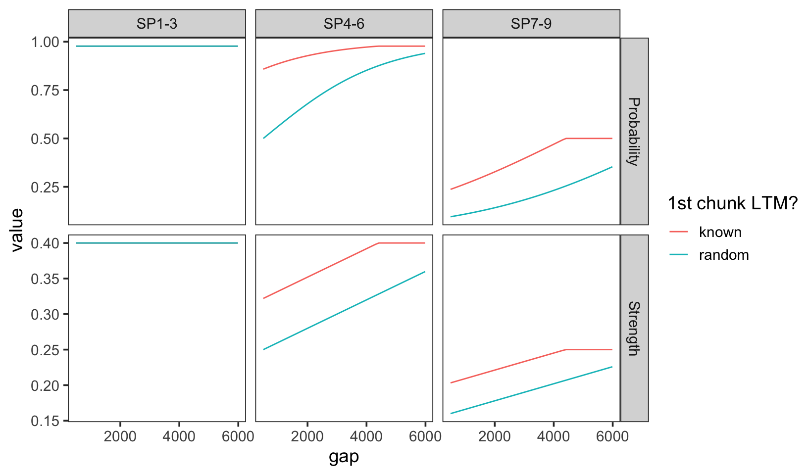
The plot below shows the predicted recall probability (top panels) and memory strength (bottom panels) as a function of the gap between the presentation of the first and second triplet of letters.
Code
library(tidyverse)library(targets)tar_source()tar_load("exp3_data_agg")plot_predictions <-function(params, data) {class(params) <-"serial_recall_pars" data |>mutate(Probability =predict(params, data, group_by =c("gap", "chunk")),Strength =predict(params, data, group_by =c("gap", "chunk"), type ="strength") ) |>pivot_longer(c(Probability, Strength), names_to ="type", values_to ="value") |>ggplot(aes(gap, value, color = chunk, group = chunk)) +geom_line() +scale_color_discrete("1st chunk LTM?") +facet_grid(type~itemtype, scales ="free") +theme_test(base_size =14)}params <-c(prop =0.4, prop_ltm =0.55, tau =0.25, gain =25, rate =0.05)plot_predictions(params, exp3_data_agg)
Look first at the bottom panels showing raw memory strength. The lines are exactly parallel until a gap ~ 4500 ms. At that point the model has recovered all the resources consumed by encoding the chunked first triplet of letters. An interaction only occurs after this, because there are still resources left to recover from encoding the random first triplet of letters.
In contrast, we see an interaction in the predicted recall probability (top panels) because the model predicts a sigmoidal relationship between memory strength and recall probability. This is a consequence of the logistic function used to map memory strength to recall probability. And as you can see, the interaction actually goes in the opposite direction when performance is low in the third tripplet.
The math
We didn’t need a simulation to tell us - we should have done simple math with the model a long time ago. Assuming no upper limit for simplicity, here is the predicted memory strength for the second tripplet:
Chunk type
Gap
Memory strength
random
shortgap
\(p \cdot (1-p + r \cdot t_{short})\)
known
shortgap
\(p \cdot (1-p \cdot p_{ltm} + r \cdot t_{short})\)
random
longgap
\(p \cdot (1-p + r \cdot t_{long})\)
known
longgap
\(p \cdot (1-p \cdot p_{ltm} + r \cdot t_{long})\)
Therefore the difference between known and random chunks separately for short and long gaps is the same:
shortgap: \(p^2 \cdot (1 - p_{ltm})\)
longgap: \(p^2 \cdot (1 - p_{ltm})\)
because the terms \(r \cdot t_{short}\) and \(r \cdot t_{long}\) cancel out if resources have not fully recovered. This is why the model predicts only additive effects of chunking and free time.
The model does predict an interaction if resources recover fully before the second tripplet is presented. But this also means that there will be no primacy effect from the first to the second tripplet, which is not what we observe in the data.
In summary, the premise on which our introduction is currently built is not supported by the model.
An interactive shiny app
I found it very useful to be able to quickly explore the model’s predictions. I created a shiny app that allows you to explore the model’s predictions for the proactive benefits of chunking and free time. You can use the sliders below to control the parameters of the model and see how the predicted probability of recall changes as a function of the conditions in the experiment.
#| standalone: true
#| viewerHeight: 700
library(shiny)
library(shinylive)
library(ggplot2)
library(dplyr)
library(tidyr)

# define functions
pred_prob <- function(
    setsize, ISI = rep(0.5, setsize), item_in_ltm = rep(TRUE, setsize),
    prop = 0.2, prop_ltm = 0.5, tau = 0.15, gain = 25, rate = 0.1,
    r_max = 1, lambda = 1, growth = "linear", type = "response") {
  R <- r_max
  strengths <- vector("numeric", length = setsize)
  p_recall <- vector("numeric", length = setsize)
  prop_ltm <- ifelse(item_in_ltm, prop_ltm, 1)

  for (item in 1:setsize) {
    # strength of the item and recall probability
    strengths[item] <- (prop * R)^lambda

    # amount of resources consumed by the item
    r_cost <- strengths[item]^(1 / lambda) * prop_ltm[item]
    R <- R - r_cost

    # recover resources
    R <- switch(growth,
      "linear" = min(r_max, R + rate * ISI[item]),
      "asy" = R + (r_max - R) * (1 - exp(-rate * ISI[item]))
    )
  }

  if (type == "response") {
    1 / (1 + exp(-(strengths - tau) * gain))
  } else {
    strengths
  }
}

predict_resmodel <- function(object, data, group_by, type = "response", ...) {
  if (missing(group_by)) {
    pred <- pred_prob(
        setsize = nrow(data),
        ISI = data$ISI,
        item_in_ltm = data$item_in_ltm,
        prop = object["prop"],
        prop_ltm = object["prop_ltm"],
        tau = object["tau"],
        gain = object["gain"],
        rate = object["rate"],
        type = type,
        ...
      )
    return(pred)
  }

  by <- do.call(paste, c(data[, group_by], sep = "_"))
  out <- lapply(split(data, by), function(x) {
    x$pred_tmp_col295 <- predict_resmodel(object, x, type = type, ...)
    x
  })
  out <- do.call(rbind, out)
  out <- suppressMessages(dplyr::left_join(data, out))
  out$pred_tmp_col295
}

data <- expand.grid(chunk = c("known", "random"),
                    gap = seq(500, 6000, by = 225),
                    itemtype = c("SP1-3", "SP4-6", "SP7-9"))

data$ISI <- ifelse(data$itemtype == "SP1-3", data$gap/1000, 0.5)
data$item_in_ltm <- ifelse(data$itemtype == "SP1-3", data$chunk == "known", FALSE)
shinyApp(
  ui = fluidPage(
    titlePanel("Interactive Plot"),
    sidebarLayout(
      sidebarPanel(
        sliderInput("prop", "prop:", min = 0, max = 1, value = 0.2),
        sliderInput("prop_ltm", "prop_ltm:", min = 0, max = 1, value = 0.55),
        sliderInput("rate", "rate:", min = 0, max = 1, value = 0.02),
        sliderInput("gain", "gain:", min = 1, max = 100, value = 25),
        sliderInput("tau", "tau:", min = 0, max = 1, value = 0.14),
      ),
      mainPanel(
        plotOutput("distPlot")
      )
    )
  ),
  server = function(input, output) {
    output$distPlot <- renderPlot({
      par <- c(prop = input$prop, prop_ltm = input$prop_ltm, rate = input$rate, gain = input$gain, tau = input$tau)
      data |>
        # TODO: can I reuse the computation?
        mutate(
          Probability = predict_resmodel(par, data = data, group_by = c("gap", "chunk")),
          Strength = predict_resmodel(par, data = data, group_by = c("gap", "chunk"), type = "strength")
        ) |>
        pivot_longer(c(Probability, Strength), names_to = "type", values_to = "value") |>
        ggplot(aes(gap, value, color = chunk, group = chunk)) +
        geom_line() +
        scale_color_discrete("1st chunk LTM?") +
        facet_grid(type~itemtype, scales = "free") +
        theme_classic(base_size = 14)
    })
  }
)
Why the best fitting model has a very low recovery?
Both in this experiment and in Mizrak & Oberauer (2022), the proactive benefit of time is global - it affects all subsequent items. With a couple of more simulations, we can see that the degree of local vs global benefit depends on the the prop depletion parameter.
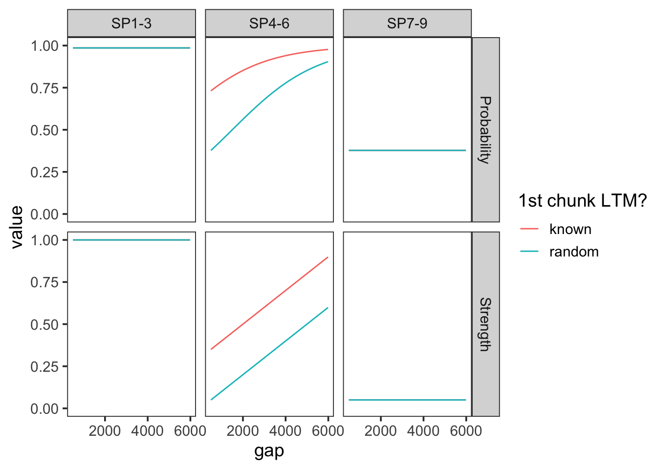
With very high prop = 1, the second tripplet will depelete all remaining resources, and then resources will be equivalent for all subsequent items. This is the most local benefit.
Code
params <-c(prop =1, prop_ltm =0.7, tau =0.15, gain =5, rate =0.1)plot_predictions(params, exp3_data_agg) +coord_cartesian(ylim =c(0, 1))
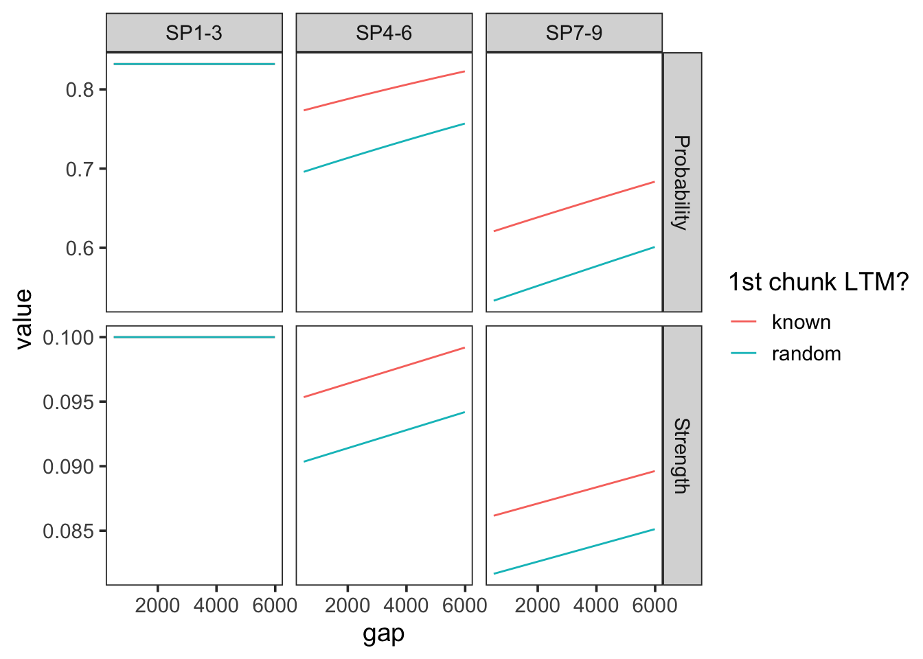
With very low prop = 0.1, the second tripplet will depelete only 10% of the remaining resources, and the proactive benefit will propagate to all subsequent items. This is the most global benefit.
Code
params <-c(prop =0.1, prop_ltm =0.5, tau =0.08, gain =80, rate =0.007)plot_predictions(params, exp3_data_agg)
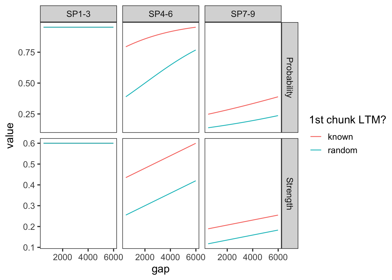
And with a middle range prop = 0.5, the second tripplet will depelete 50% of the remaining resources, and preserving some of the proactive benefit, but reducing it for subsequent items:
Code
params <-c(prop =0.6, prop_ltm =0.5, tau =0.3, gain =10, rate =0.05)plot_predictions(params, exp3_data_agg)
So what?
since we see mostly a global benefit in the data, in order for the model to fit well, it estimates a very low depletion rate (~ 0.2). But then to account for the primacy effect, and to prevent full recovery of resources between items with such low depletion, it also needs to estimate a very low recovery rate. Thus, all of our fits having slow recovery rates, are not related to accounting for the small interaction between chunking and free time, but rather to account for the global proactive benefits and primacy.
---title: "Exploring model predictions"format: htmldate: 05/20/2024date-modified: last-modifiedfilters: - shinylive---## OverviewThe motivation for the paper was based on the assumption that the resource model should predict an interaction between the proactive benefits of free time and chunking:> "If the LTM benefit arises because encoding a chunk consumes less of an encoding resource, then that benefit should diminish with longer free time, because over time the resource grows back towards its maximal level regardless of how much of it has been consumed by encoding the initial triplet of letters. "As we discussed, I was not sure if the model actually predicts this. Exploring the model's predictions for the *memory strength* latent variable reveals that this is not what the model predicts. As long as resources have not recovered to their maximum level, the model predicts only *additive* effects of chunking and free time.## An exampleThe plot below shows the predicted recall probability (top panels) and memory strength (bottom panels) as a function of the gap between the presentation of the first and second triplet of letters. ```{r}#| message: false#| fig.width: 8.5#| fig.height: 5library(tidyverse)library(targets)tar_source()tar_load("exp3_data_agg")plot_predictions <-function(params, data) {class(params) <-"serial_recall_pars" data |>mutate(Probability =predict(params, data, group_by =c("gap", "chunk")),Strength =predict(params, data, group_by =c("gap", "chunk"), type ="strength") ) |>pivot_longer(c(Probability, Strength), names_to ="type", values_to ="value") |>ggplot(aes(gap, value, color = chunk, group = chunk)) +geom_line() +scale_color_discrete("1st chunk LTM?") +facet_grid(type~itemtype, scales ="free") +theme_test(base_size =14)}params <-c(prop =0.4, prop_ltm =0.55, tau =0.25, gain =25, rate =0.05)plot_predictions(params, exp3_data_agg)```Look first at the bottom panels showing raw memory strength. The lines are exactly parallel until a gap ~ 4500 ms. At that point the model has recovered all the resources consumed by encoding the *chunked* first triplet of letters. An interaction only occurs after this, because there are still resources left to recover from encoding the *random* first triplet of letters.In contrast, we see an interaction in the predicted *recall probability* (top panels) because the model predicts a sigmoidal relationship between memory strength and recall probability. This is a consequence of the logistic function used to map memory strength to recall probability. And as you can see, the interaction actually goes in the opposite direction when performance is low in the third tripplet.## The mathWe didn't need a simulation to tell us - we should have done simple math with the model a long time ago. Assuming no upper limit for simplicity, here is the predicted memory strength for the second tripplet: | Chunk type | Gap | Memory strength | |------------|-----|-----------------| | random | shortgap | $p \cdot (1-p + r \cdot t_{short})$ | | known | shortgap | $p \cdot (1-p \cdot p_{ltm} + r \cdot t_{short})$ | | random | longgap | $p \cdot (1-p + r \cdot t_{long})$ | | known | longgap | $p \cdot (1-p \cdot p_{ltm} + r \cdot t_{long})$ |Therefore the difference between known and random chunks separately for short and long gaps is the same: - shortgap: $p^2 \cdot (1 - p_{ltm})$ - longgap: $p^2 \cdot (1 - p_{ltm})$because the terms $r \cdot t_{short}$ and $r \cdot t_{long}$ cancel out if resources have not fully recovered. This is why the model predicts only additive effects of chunking and free time.The model does predict an interaction if resources recover fully before the second tripplet is presented. But this also means that there will be no primacy effect from the first to the second tripplet, which is not what we observe in the data.In summary, the premise on which our introduction is currently built is not supported by the model.## An interactive shiny appI found it very useful to be able to quickly explore the model's predictions. I created a shiny app that allows you to explore the model's predictions for the proactive benefits of chunking and free time. You can use the sliders below to control the parameters of the model and see how the predicted probability of recall changes as a function of the conditions in the experiment.::: {.column-page-right}```{shinylive-r}#| standalone: true#| viewerHeight: 700library(shiny)library(shinylive)library(ggplot2)library(dplyr)library(tidyr)# define functionspred_prob <- function( setsize, ISI = rep(0.5, setsize), item_in_ltm = rep(TRUE, setsize), prop = 0.2, prop_ltm = 0.5, tau = 0.15, gain = 25, rate = 0.1, r_max = 1, lambda = 1, growth = "linear", type = "response") { R <- r_max strengths <- vector("numeric", length = setsize) p_recall <- vector("numeric", length = setsize) prop_ltm <- ifelse(item_in_ltm, prop_ltm, 1) for (item in 1:setsize) { # strength of the item and recall probability strengths[item] <- (prop * R)^lambda # amount of resources consumed by the item r_cost <- strengths[item]^(1 / lambda) * prop_ltm[item] R <- R - r_cost # recover resources R <- switch(growth, "linear" = min(r_max, R + rate * ISI[item]), "asy" = R + (r_max - R) * (1 - exp(-rate * ISI[item])) ) } if (type == "response") { 1 / (1 + exp(-(strengths - tau) * gain)) } else { strengths }}predict_resmodel <- function(object, data, group_by, type = "response", ...) { if (missing(group_by)) { pred <- pred_prob( setsize = nrow(data), ISI = data$ISI, item_in_ltm = data$item_in_ltm, prop = object["prop"], prop_ltm = object["prop_ltm"], tau = object["tau"], gain = object["gain"], rate = object["rate"], type = type, ... ) return(pred) } by <- do.call(paste, c(data[, group_by], sep = "_")) out <- lapply(split(data, by), function(x) { x$pred_tmp_col295 <- predict_resmodel(object, x, type = type, ...) x }) out <- do.call(rbind, out) out <- suppressMessages(dplyr::left_join(data, out)) out$pred_tmp_col295}data <- expand.grid(chunk = c("known", "random"), gap = seq(500, 6000, by = 225), itemtype = c("SP1-3", "SP4-6", "SP7-9"))data$ISI <- ifelse(data$itemtype == "SP1-3", data$gap/1000, 0.5)data$item_in_ltm <- ifelse(data$itemtype == "SP1-3", data$chunk == "known", FALSE) shinyApp( ui = fluidPage( titlePanel("Interactive Plot"), sidebarLayout( sidebarPanel( sliderInput("prop", "prop:", min = 0, max = 1, value = 0.2), sliderInput("prop_ltm", "prop_ltm:", min = 0, max = 1, value = 0.55), sliderInput("rate", "rate:", min = 0, max = 1, value = 0.02), sliderInput("gain", "gain:", min = 1, max = 100, value = 25), sliderInput("tau", "tau:", min = 0, max = 1, value = 0.14), ), mainPanel( plotOutput("distPlot") ) ) ), server = function(input, output) { output$distPlot <- renderPlot({ par <- c(prop = input$prop, prop_ltm = input$prop_ltm, rate = input$rate, gain = input$gain, tau = input$tau) data |> # TODO: can I reuse the computation? mutate( Probability = predict_resmodel(par, data = data, group_by = c("gap", "chunk")), Strength = predict_resmodel(par, data = data, group_by = c("gap", "chunk"), type = "strength") ) |> pivot_longer(c(Probability, Strength), names_to = "type", values_to = "value") |> ggplot(aes(gap, value, color = chunk, group = chunk)) + geom_line() + scale_color_discrete("1st chunk LTM?") + facet_grid(type~itemtype, scales = "free") + theme_classic(base_size = 14) }) })```:::## Why the best fitting model has a very low recovery?Both in this experiment and in Mizrak & Oberauer (2022), the proactive benefit of time is global - it affects all subsequent items. With a couple of more simulations, we can see that the degree of local vs global benefit depends on the the `prop` depletion parameter. ---With very high `prop = 1`, the second tripplet will depelete all remaining resources, and then resources will be equivalent for all subsequent items. This is the most local benefit.```{r}params <-c(prop =1, prop_ltm =0.7, tau =0.15, gain =5, rate =0.1)plot_predictions(params, exp3_data_agg) +coord_cartesian(ylim =c(0, 1))```---With very low `prop = 0.1`, the second tripplet will depelete only 10% of the *remaining resources*, and the proactive benefit will propagate to all subsequent items. This is the most global benefit.```{r}params <-c(prop =0.1, prop_ltm =0.5, tau =0.08, gain =80, rate =0.007)plot_predictions(params, exp3_data_agg) ```---And with a middle range `prop = 0.5`, the second tripplet will depelete 50% of the *remaining resources*, and preserving some of the proactive benefit, but reducing it for subsequent items:```{r}params <-c(prop =0.6, prop_ltm =0.5, tau =0.3, gain =10, rate =0.05)plot_predictions(params, exp3_data_agg)```### So what?since we see mostly a global benefit in the data, in order for the model to fit well, it estimates a very low depletion rate (~ 0.2). But then to account for the primacy effect, and to prevent full recovery of resources between items with such low depletion, it also needs to estimate a very low recovery rate. Thus, all of our fits having slow recovery rates, are not related to accounting for the small interaction between chunking and free time, but rather to account for the global proactive benefits and primacy.