In Exploring model predictions I used a shiny app to understand how the basic model with linear resource recovery works, and I found that it does not predict an interaction between chunking and free time proactive benefits. I suspect that a model with a non-linear recovery will be different, because for a fixed time interval it will recover more resource the lower the resource level is. Let’s explore this. Resources are recovered according to the following equation:
where \(R_{\text{max}}\) is the maximum resource level, \(R_{\text{current}}\) is the current resource level, \(\text{rate}\) is the recovery rate, and \(t\) is the time elapsed.
Just the resource recovery
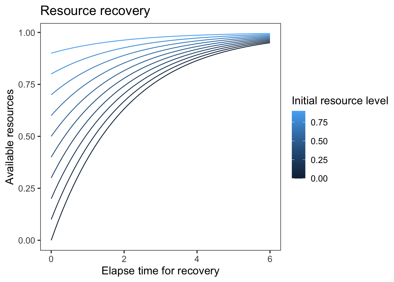
Plot the amount of resource recovered for a fixed time interval as a function of the current resource level.
Here’s a fixed plot for rate = 0.5:
Code
resources <-function(R, rate, time, r_max =1) { (r_max - R) * (1-exp(-rate * time))}pars <-expand.grid(R =seq(0, 0.9, by =0.1), time =seq(0, 6, by =0.1))pars$resources <-resources(pars$R, 0.5, pars$time)# ggplot with rate as frame and then convert via ggplotly to an interactive plotlibrary(ggplot2)ggplot(pars, aes(time, resources + R, color = R, group = R)) +geom_line() +theme_test(base_size =14) +labs(title ="Resource recovery",x ="Elapse time for recovery",y ="Available resources",color ="Initial resource level" )
Yes, now we can clearly see above that within the same time interval, the lower the resource level, the more resources are recovered. Let’s see if this produces the interaction we expected.
Model predictions
#| standalone: true
#| viewerHeight: 700
library(shiny)
library(shinylive)
library(ggplot2)
library(dplyr)
library(tidyr)

# define functions
pred_prob <- function(
    setsize, ISI = rep(0.5, setsize), item_in_ltm = rep(TRUE, setsize),
    prop = 0.2, prop_ltm = 0.5, tau = 0.15, gain = 25, rate = 0.1,
    r_max = 1, lambda = 1, growth = "linear", type = "response") {
  R <- r_max
  strengths <- vector("numeric", length = setsize)
  p_recall <- vector("numeric", length = setsize)
  prop_ltm <- ifelse(item_in_ltm, prop_ltm, 1)

  for (item in 1:setsize) {
    # strength of the item and recall probability
    strengths[item] <- (prop * R)^lambda

    # amount of resources consumed by the item
    r_cost <- strengths[item]^(1 / lambda) * prop_ltm[item]
    R <- R - r_cost

    # recover resources
    R <- switch(growth,
      "linear" = min(r_max, R + rate * ISI[item]),
      "asy" = R + (r_max - R) * (1 - exp(-rate * ISI[item]))
    )
  }

  if (type == "response") {
    1 / (1 + exp(-(strengths - tau) * gain))
  } else {
    strengths
  }
}

predict_resmodel <- function(object, data, group_by, type = "response", ...) {
  if (missing(group_by)) {
    pred <- pred_prob(
      setsize = nrow(data),
      ISI = data$ISI,
      item_in_ltm = data$item_in_ltm,
      prop = object["prop"],
      prop_ltm = object["prop_ltm"],
      tau = object["tau"],
      gain = object["gain"],
      rate = object["rate"],
      type = type,
      ...
    )
    return(pred)
  }

  by <- do.call(paste, c(data[, group_by], sep = "_"))
  out <- lapply(split(data, by), function(x) {
    x$pred_tmp_col295 <- predict_resmodel(object, x, type = type, ...)
    x
  })
  out <- do.call(rbind, out)
  out <- suppressMessages(dplyr::left_join(data, out))
  out$pred_tmp_col295
}

data <- expand.grid(
  chunk = c("known", "random"),
  gap = seq(500, 6000, by = 225),
  itemtype = c("SP1-3", "SP4-6", "SP7-9")
)

data$ISI <- ifelse(data$itemtype == "SP1-3", data$gap / 1000, 0.5)
data$item_in_ltm <- ifelse(data$itemtype == "SP1-3", data$chunk == "known", FALSE)
shinyApp(
  ui = fluidPage(
    titlePanel("Interactive Plot"),
    sidebarLayout(
      sidebarPanel(
        sliderInput("prop", "prop:", min = 0, max = 1, value = 0.15),
        sliderInput("prop_ltm", "prop_ltm:", min = 0, max = 1, value = 0.5),
        sliderInput("rate", "rate:", min = 0, max = 1, value = 0.25),
        sliderInput("gain", "gain:", min = 1, max = 100, value = 33),
        sliderInput("tau", "tau:", min = 0, max = 1, value = 0.12),
      ),
      mainPanel(
        plotOutput("distPlot")
      )
    )
  ),
  server = function(input, output) {
    output$distPlot <- renderPlot({
      par <- c(prop = input$prop, prop_ltm = input$prop_ltm, rate = input$rate, gain = input$gain, tau = input$tau)
      data |>
        mutate(
          Probability = predict_resmodel(par, data = data, group_by = c("gap", "chunk"), growth = "asy", lambda = 1),
          Strength = predict_resmodel(par, data = data, group_by = c("gap", "chunk"), type = "strength", growth = "asy", lambda = 1)
        ) |>
        pivot_longer(c(Probability, Strength), names_to = "type", values_to = "value") |>
        ggplot(aes(gap, value, color = chunk, group = chunk)) +
        geom_line() +
        scale_color_discrete("1st chunk LTM?") +
        facet_grid(type ~ itemtype, scales = "free") +
        theme_classic(base_size = 14)
    })
  }
)
With the non-linear resource recovery, we do predict an interaction between chunking and free time proactive benefits. In contrast to the linear recovery model, this interaction occurs for a large range of parameter values and does not require that resources are depleted completely in one condition in order for the interaction to occur.
---title: "Explore model predictions"format: htmldate: 05/20/2024date-modified: last-modifiedfilters: - shinylive---## Non-linear resource recovery modelIn [Exploring model predictions](model-explore.qmd) I used a shiny app to understand how the basic model with linear resource recovery works, and I found that it does not predict an interaction between chunking and free time proactive benefits. I suspect that a model with a non-linear recovery will be different, because for a fixed time interval it will recover more resource the lower the resource level is. Let's explore this. Resources are recovered according to the following equation:$$R(t) = R_{\text{current}} + (R_{\text{max}} - R_{\text{current}})(1 - e^{-\text{rate} \times t})$$where $R_{\text{max}}$ is the maximum resource level, $R_{\text{current}}$ is the current resource level, $\text{rate}$ is the recovery rate, and $t$ is the time elapsed.## Just the resource recoveryPlot the amount of resource recovered for a fixed time interval as a function of the current resource level. Here's a fixed plot for rate = 0.5:```{r resource-recovery-fixed}#| message: falseresources <- function(R, rate, time, r_max = 1) { (r_max - R) * (1 - exp(-rate * time))}pars <- expand.grid(R = seq(0, 0.9, by = 0.1), time = seq(0, 6, by = 0.1))pars$resources <- resources(pars$R, 0.5, pars$time)# ggplot with rate as frame and then convert via ggplotly to an interactive plotlibrary(ggplot2)ggplot(pars, aes(time, resources + R, color = R, group = R)) + geom_line() + theme_test(base_size = 14) + labs( title = "Resource recovery", x = "Elapse time for recovery", y = "Available resources", color = "Initial resource level" )```<br>Yes, now we can clearly see above that within the same time interval, the lower the resource level, the more resources are recovered. Let's see if this produces the interaction we expected.## Model predictions::: {.column-page-right}```{shinylive-r}#| standalone: true#| viewerHeight: 700library(shiny)library(shinylive)library(ggplot2)library(dplyr)library(tidyr)# define functionspred_prob <- function( setsize, ISI = rep(0.5, setsize), item_in_ltm = rep(TRUE, setsize), prop = 0.2, prop_ltm = 0.5, tau = 0.15, gain = 25, rate = 0.1, r_max = 1, lambda = 1, growth = "linear", type = "response") { R <- r_max strengths <- vector("numeric", length = setsize) p_recall <- vector("numeric", length = setsize) prop_ltm <- ifelse(item_in_ltm, prop_ltm, 1) for (item in 1:setsize) { # strength of the item and recall probability strengths[item] <- (prop * R)^lambda # amount of resources consumed by the item r_cost <- strengths[item]^(1 / lambda) * prop_ltm[item] R <- R - r_cost # recover resources R <- switch(growth, "linear" = min(r_max, R + rate * ISI[item]), "asy" = R + (r_max - R) * (1 - exp(-rate * ISI[item])) ) } if (type == "response") { 1 / (1 + exp(-(strengths - tau) * gain)) } else { strengths }}predict_resmodel <- function(object, data, group_by, type = "response", ...) { if (missing(group_by)) { pred <- pred_prob( setsize = nrow(data), ISI = data$ISI, item_in_ltm = data$item_in_ltm, prop = object["prop"], prop_ltm = object["prop_ltm"], tau = object["tau"], gain = object["gain"], rate = object["rate"], type = type, ... ) return(pred) } by <- do.call(paste, c(data[, group_by], sep = "_")) out <- lapply(split(data, by), function(x) { x$pred_tmp_col295 <- predict_resmodel(object, x, type = type, ...) x }) out <- do.call(rbind, out) out <- suppressMessages(dplyr::left_join(data, out)) out$pred_tmp_col295}data <- expand.grid( chunk = c("known", "random"), gap = seq(500, 6000, by = 225), itemtype = c("SP1-3", "SP4-6", "SP7-9"))data$ISI <- ifelse(data$itemtype == "SP1-3", data$gap / 1000, 0.5)data$item_in_ltm <- ifelse(data$itemtype == "SP1-3", data$chunk == "known", FALSE)shinyApp( ui = fluidPage( titlePanel("Interactive Plot"), sidebarLayout( sidebarPanel( sliderInput("prop", "prop:", min = 0, max = 1, value = 0.15), sliderInput("prop_ltm", "prop_ltm:", min = 0, max = 1, value = 0.5), sliderInput("rate", "rate:", min = 0, max = 1, value = 0.25), sliderInput("gain", "gain:", min = 1, max = 100, value = 33), sliderInput("tau", "tau:", min = 0, max = 1, value = 0.12), ), mainPanel( plotOutput("distPlot") ) ) ), server = function(input, output) { output$distPlot <- renderPlot({ par <- c(prop = input$prop, prop_ltm = input$prop_ltm, rate = input$rate, gain = input$gain, tau = input$tau) data |> mutate( Probability = predict_resmodel(par, data = data, group_by = c("gap", "chunk"), growth = "asy", lambda = 1), Strength = predict_resmodel(par, data = data, group_by = c("gap", "chunk"), type = "strength", growth = "asy", lambda = 1) ) |> pivot_longer(c(Probability, Strength), names_to = "type", values_to = "value") |> ggplot(aes(gap, value, color = chunk, group = chunk)) + geom_line() + scale_color_discrete("1st chunk LTM?") + facet_grid(type ~ itemtype, scales = "free") + theme_classic(base_size = 14) }) })```:::With the non-linear resource recovery, we do predict an interaction between chunking and free time proactive benefits. In contrast to the linear recovery model, this interaction occurs for a large range of parameter values and does not require that resources are depleted completely in one condition in order for the interaction to occur.