Code
library(tidyverse)
library(targets)
library(GGally)
library(kableExtra)
# load "R/*" scripts and saved R objects from the targets pi
tar_source()
tar_load(c(exp1_data, exp2_data, exp1_data_agg, exp2_data_agg, exp3_data_agg))
set.seed(213)Fit the non-linear resource recovery model to the three experiments. Dashed lines are model predictions. Solid dots are the observed data and solid lines are linear regression lines.
library(tidyverse)
library(targets)
library(GGally)
library(kableExtra)
# load "R/*" scripts and saved R objects from the targets pi
tar_source()
tar_load(c(exp1_data, exp2_data, exp1_data_agg, exp2_data_agg, exp3_data_agg))
set.seed(213)start <- c(prop = 0.15, prop_ltm = 0.5, rate = 0.25, gain = 30, tau = 0.12)
est1 <- estimate_model(start, data = exp1_data_agg, exclude_sp1 = TRUE, growth = "asy")
exp1_data_agg$pred <- predict(est1, exp1_data_agg, group_by = c("chunk", "gap"), growth = "asy")
exp1_data_agg |>
ggplot(aes(x = gap, y = p_correct, color = chunk)) +
geom_point() +
geom_line() +
geom_line(aes(y = pred), linetype = "dashed") +
scale_color_discrete("First chunk LTM?") +
facet_wrap(~itemtype)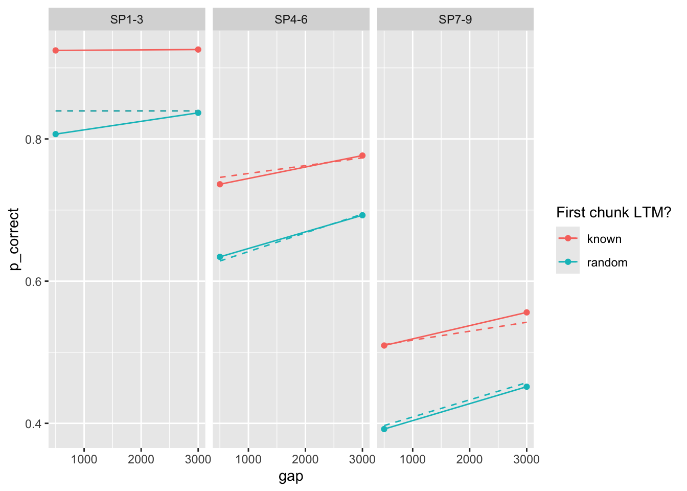
est2 <- estimate_model(est1$par, data = exp2_data_agg, exclude_sp1 = TRUE, growth = "asy")
exp2_data_agg$pred <- predict(est2, exp2_data_agg, group_by = c("chunk", "gap"), growth = "asy")
exp2_data_agg |>
  ggplot(aes(x = gap, y = p_correct, color = chunk)) +
  geom_point() +
  geom_line() +
  geom_line(aes(y = pred), linetype = "dashed") +
  scale_color_discrete("First chunk LTM?") +
  facet_wrap(~itemtype)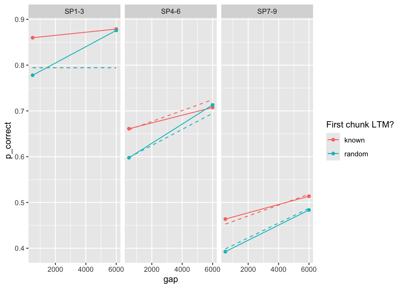
est3 <- estimate_model(est1$par, data = exp3_data_agg, exclude_sp1 = TRUE, growth = "asy")
exp3_data_agg$pred <- predict(est3, exp3_data_agg, group_by = c("chunk", "gap"), growth = "asy")
exp3_data_agg |>
  ggplot(aes(x = gap, y = p_correct, color = chunk)) +
  geom_point(alpha = 0.5) +
  stat_smooth(method = "lm", se = FALSE, linewidth = 0.5) +
  geom_line(aes(y = pred), linetype = "dashed", linewidth = 1.1) +
  scale_color_discrete("First chunk LTM?") +
  facet_wrap(~itemtype)
`geom_smooth()` using formula = 'y ~ x'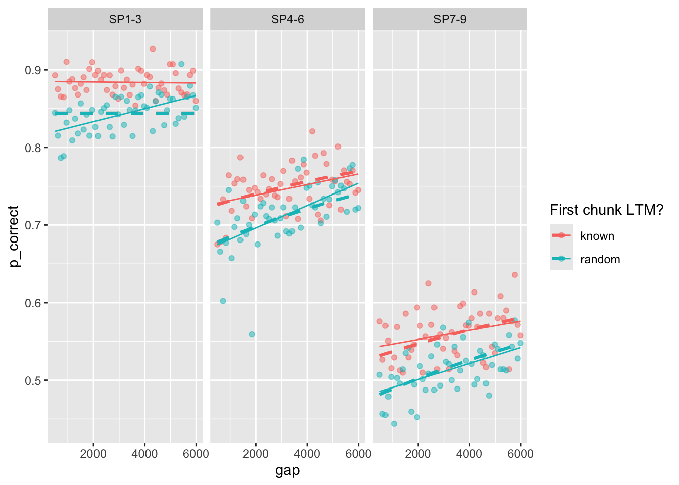
parameter estimates for the three experiments:
kable(round(bind_rows(est1$par, est2$par, est3$par), 3)) %>%
kable_styling()| prop | prop_ltm | rate | gain | tau |
|---|---|---|---|---|
| 0.112 | 0.511 | 0.121 | 95.703 | 0.095 |
| 0.103 | 0.726 | 0.107 | 93.932 | 0.089 |
| 0.106 | 0.754 | 0.070 | 87.741 | 0.086 |
With the non-linear recovery model, we get rate estiates of 0.121, 0.107, 0.070 in the three experiments. Unlike the linear recovery rate, we cannot interpret these simply. But we can ask, given the resource recovery equation and these estimates, how long will it take to recover a proportion X of the resource from 0? This is equivalent to the equation
\[ 1-e^{-rate \times t} = X \]
solving for t gives
\[ t = -\frac{log(1-X)}{rate} \]
which we can plot:
rdata <- expand.grid(
  X = seq(0.1, 0.9, 0.1),
  rates = round(c(est1$par["rate"], est2$par["rate"], est3$par["rate"]), 3)
)

rdata$time <- -log(1 - rdata$X) / rdata$rates

rdata |>
  ggplot(aes(x = X, y = time, color = factor(rates))) +
  geom_line() +
  scale_color_discrete("Rate") +
  labs(x = "Proportion recovered", y = "Time to recover")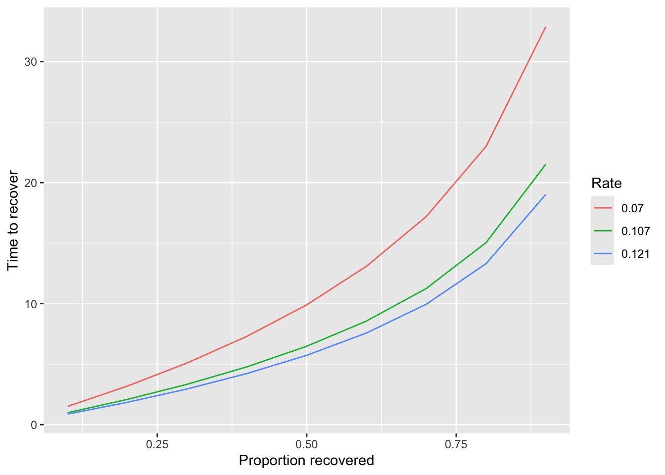
We see that it takes: