Distribution functions for the Interference Measurement Model (IMM)

Density, distribution, and random generation functions for the interference measurement model with the location of mu, strength of cue- dependent activation c, strength of cue-independent activation a, the generalization gradient s, and the precision of memory representations kappa.

Usage

dimm(
  x,
  mu = c(0, 2, -1.5),
  dist = c(0, 0.5, 2),
  c = 5,
  a = 2,
  b = 1,
  s = 2,
  kappa = 5,
  log = FALSE
)

pimm(
  q,
  mu = c(0, 2, -1.5),
  dist = c(0, 0.5, 2),
  c = 1,
  a = 0.2,
  b = 0,
  s = 2,
  kappa = 5
)

qimm(
  p,
  mu = c(0, 2, -1.5),
  dist = c(0, 0.5, 2),
  c = 1,
  a = 0.2,
  b = 0,
  s = 2,
  kappa = 5
)

rimm(
  n,
  mu = c(0, 2, -1.5),
  dist = c(0, 0.5, 2),
  c = 1,
  a = 0.2,
  b = 1,
  s = 2,
  kappa = 5
)

Arguments

x

Vector of observed responses

mu

Vector of locations

dist

Vector of distances of the item locations to the cued location

c

Vector of strengths for cue-dependent activation

a

Vector of strengths for cue-independent activation

b

Vector of baseline activation

s

Vector of generalization gradients

kappa

Vector of precision values

log

Logical; if TRUE, values are returned on the log scale.

q

Vector of quantiles

p

Vector of probability

n

Number of observations to generate data for

Value

dimm gives the density of the interference measurement model, pimm gives the cumulative distribution function of the interference measurement model, qimm gives the quantile function of the interference measurement model, and rimm gives the random generation function for the interference measurement model.

References

Oberauer, K., Stoneking, C., Wabersich, D., & Lin, H.-Y. (2017). Hierarchical Bayesian measurement models for continuous reproduction of visual features from working memory. Journal of Vision, 17(5), 11.

Examples

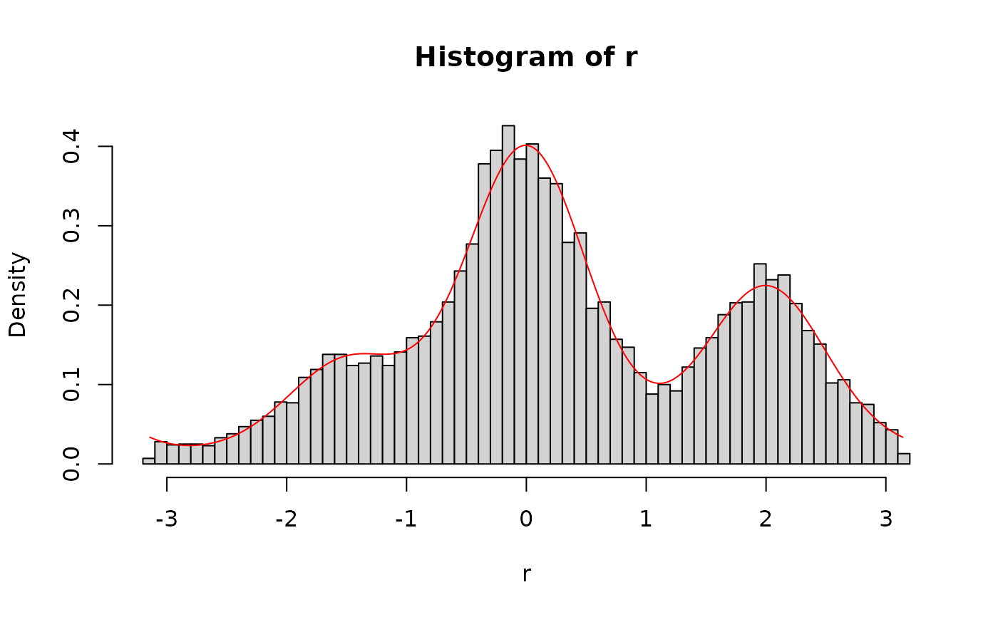
# generate random samples from the imm and overlay the density
r <- rimm(10000, mu = c(0, 2, -1.5), dist = c(0, 0.5, 2),
          c = 5, a = 2, s = 2, b = 1, kappa = 4)
x <- seq(-pi,pi,length.out=10000)
d <- dimm(x, mu = c(0, 2, -1.5), dist = c(0, 0.5, 2),
          c = 5, a = 2, s = 2, b = 1, kappa = 4)
hist(r, breaks=60, freq=FALSE)
lines(x,d,type="l", col="red")