The EZ-Diffusion Model (EZDM)
Gidon Frischkorn
Ven Popov
Source:vignettes/articles/bmm_ezdm.Rmd
bmm_ezdm.Rmd1 Introduction to the model
The diffusion model (Ratcliff 1978) is a widely used model in speeded decision-making. It describes how participants accumulate noisy evidence over time until reaching one of two decision boundaries. Usually, the diffusion model is fit to trial-level reaction time distributions, which can be computationally intensive, especially for hierarchical Bayesian estimation.
The EZ-Diffusion Model (Wagenmakers, Van Der Maas, and Grasman 2007) provides a simplified alternative building on closed-form equations that relate the parameters of the diffusion model to easily computed summary statistics: mean reaction time (MRT), reaction time variance (VRT), and accuracy (proportion correct, Pc). This makes it possible to calculate diffusion model parameters from aggregated data without fitting to individual trials.
1.1 The Diffusion Model
In the standard diffusion model, evidence accumulates from a starting point toward one of two boundaries. The key parameters are:
- Drift rate (\(v\)): The average rate of evidence accumulation, reflecting task difficulty or ability
- Boundary separation (\(a\)): The distance between the two decision boundaries, reflecting the speed-accuracy tradeoff
- Non-decision time (\(T_{er}\)): Time for processes outside the decision (encoding, motor response)
- Starting point (\(z\)): A response bias indicating where evidence accumulation begins relative to the boundaries
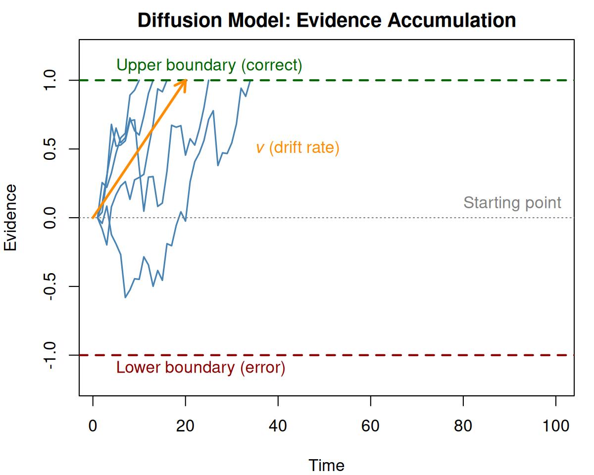
Figure 1.1: Illustration of the diffusion model. Evidence accumulates from the starting point until reaching the upper (correct) or lower (error) boundary.
1.2 The EZ Equations
Wagenmakers, Van Der Maas, and Grasman (2007) provided closed-form solutions relating the diffusion model parameters to observable summary statistics. For the 3-parameter version (assuming symmetric starting point, \(z = a/2\)):
Given the proportion correct (\(P_c\)), mean RT of correct responses (\(MRT\)), and variance of correct RTs (\(VRT\)), the parameters can be computed as:
\[ v = \text{sign}(P_c - 0.5) \cdot s \cdot \left[ L(P_c) \cdot \frac{P_c^2 L(P_c) - P_c \cdot L(P_c) + P_c - 0.5}{VRT} \right]^{1/4} \]
\[ a = s^2 \cdot \frac{L(P_c)}{v} \]
\[ T_{er} = MRT - \frac{a}{2v} \cdot \frac{1 - e^{-\frac{va}{s^2}}}{1 + e^{-\frac{va}{s^2}}} \]
where \(L(P_c) = \ln\left(\frac{P_c}{1 - P_c}\right)\) is the logit function and \(s\) is the diffusion constant (typically fixed to 1 for identification).
1.3 The 4-Parameter Extension
The original EZ model assumes a symmetric starting point. Srivastava, Holmes, and Simen (2016) derived the moments of first-passage times for the Wiener diffusion process with arbitrary starting points, enabling a 4-parameter version that can estimate starting point bias (\(z_r\), the relative starting point). This 4-parameter version, however, requires separate summary statistics for responses to each boundary:
- Mean and variance of RTs for upper boundary responses (typically correct)
- Mean and variance of RTs for lower boundary responses (typically errors)
With sufficient responses at both the upper and lower bound, this allows estimation of response bias, which is important when participants favor one response over another.
1.4 Bayesian Estimation
So far, studies using the EZ-Diffusion model have adopted step-wise analyses approaches. First, diffusion model parameters are calculated for summary statistics for each individual in each design cell. Second, the calculated parameters are submitted to statistical tests evaluating differences between experimental conditions. This approach has two downsides: 1) uncertainty in parameter estimation is not sufficiently propagated between analysis steps, and 2) all parameters of the diffusion model were allowed to vary over all design cells, bearing the risk of over fitting. To address these issues, Chávez De la Peña and Vandekerckhove (2025) introduced a Bayesian hierarchical approach to the EZ-diffusion model. This approach combines the derivation of summary statistics from diffusion model parameters with a probabilistic model of the sampling distributions of the summary statistics. Specifically, this approach:
- Treats the summary statistics as observed data generated from a known sampling distribution
- Uses likelihood-based inference to estimate parameters with proper uncertainty quantification
- Enables hierarchical modeling with random effects across participants
Chávez De la Peña and Vandekerckhove (2025) shared JAGS code alongside their model. The downside of this implementation is that the model code has to be adapted to different experimental designs which likely leads to errors and increases the bar for using the implementation. The bmm package implements this Bayesian approach, allowing researchers to:
- Estimate uncertainty in parameter estimates
- Include random effects for participants
- Compare conditions using Bayesian hypothesis testing
- Leverage the full power of the
brmsmodeling framework
2 Parametrization in the bmm package
The bmm package implements two versions of the EZ-diffusion model:
2.1 3-Parameter Version (version = "3par")
Estimates three parameters with a fixed symmetric starting point (\(z_r = 0.5\)):
| Parameter | Description | Link Function |
|---|---|---|
drift |
Drift rate (\(v\)) - rate of evidence accumulation | identity |
bound |
Boundary separation (\(a\)) - response caution | log |
ndt |
Non-decision time (\(T_{er}\)) - encoding + motor time | log |
The diffusion constant s is fixed to 1 for identification.
2.2 4-Parameter Version (version = "4par")
Adds estimation of starting point bias:
| Parameter | Description | Link Function |
|---|---|---|
drift |
Drift rate (\(v\)) | identity |
bound |
Boundary separation (\(a\)) | log |
ndt |
Non-decision time (\(T_{er}\)) | log |
zr |
Relative starting point (0-1 scale) | logit |
Note that zr = 0.5 indicates no bias (symmetric starting point), zr > 0.5 indicates bias toward the upper boundary, and zr < 0.5 indicates bias toward the lower boundary.
3 Data requirements
Unlike other models in bmm that work with trial-level data, the EZ-diffusion model requires aggregated summary statistics:
| Variable | Description |
|---|---|
mean_rt |
Mean reaction time (in seconds) |
var_rt |
Variance of reaction times |
n_upper |
Number of responses hitting the upper boundary |
n_trials |
Total number of trials |
For the 3-parameter version, mean_rt and var_rt should be computed from all correct responses pooled together.
For the 4-parameter version, you need separate statistics for upper and lower boundary responses:
- mean_rt_upper, var_rt_upper for upper boundary (correct) responses
- mean_rt_lower, var_rt_lower for lower boundary (error) responses
4 Preparing data with ezdm_summary_stats()
The bmm package provides the ezdm_summary_stats() function to compute the required aggregated statistics from trial-level RT data in the correct format. This function addresses a critical challenge in applying the EZ-Diffusion Model: RT contaminants (fast guesses, lapses, attentional failures) can severely distort mean and variance estimates, leading to biased parameter estimates (Wagenmakers et al. 2008).
4.1 Why Robust Estimation Matters
Research by Wagenmakers et al. (2008) demonstrated that contaminant responses systematically bias EZ-DM parameter estimates. Even a small proportion (5-10%) of outlier RTs can substantially affect the moments used to compute drift rate, boundary, and non-decision time. To illustrate this, let’s generate trial-level data with known parameters and introduce realistic contaminants:
library(bmm)
library(rtdists)
library(dplyr)

set.seed(42)

# Generate clean trial-level data with known parameters
n_trials <- 200
true_drift <- 2.5
true_bound <- 1.2
true_ndt <- 0.25

# Simulate diffusion process
trials_clean <- rdiffusion(
  n = n_trials,
  a = true_bound,
  v = true_drift,
  t0 = true_ndt,
  z = 0.5 * true_bound  # Symmetric starting point
)

# Add contaminants (5% fast guesses and lapses uniformly distributed between 0.1 and 3 seconds)
n_contaminants <- round(n_trials * 0.05)
contaminant_idx <- sample(n_trials, n_contaminants)

trials_contaminated <- trials_clean
trials_contaminated$rt[contaminant_idx] <- runif(n_contaminants, 0.1, 3)
trials_contaminated$response[contaminant_idx] <- sample(c("upper", "lower"),
                                                         n_contaminants,
                                                         replace = TRUE)

# Convert to format expected by ezdm_summary_stats
trials_contaminated <- trials_contaminated %>%
  mutate(
    correct = as.numeric(response == "upper"),
    subject = 1,
    condition = "standard"
  )

# Compare moments
cat("Clean data:       Mean RT =",
    round(mean(trials_clean$rt[trials_clean$response == "upper"]), 3),
    ", Var RT =",
    round(var(trials_clean$rt[trials_clean$response == "upper"]), 4), "\n")
#> Clean data:       Mean RT = 0.476 , Var RT = 0.0205
cat("Contaminated data: Mean RT =",
    round(mean(trials_contaminated$rt[trials_contaminated$correct == 1]), 3),
    ", Var RT =",
    round(var(trials_contaminated$rt[trials_contaminated$correct == 1]), 4), "\n")
#> Contaminated data: Mean RT = 0.514 , Var RT = 0.0756
The contaminants substantially reduce both the mean and variance of correct RTs, which would lead to biased parameter estimates if we used simple moments.
4.2 Three Methods for Computing Statistics
The ezdm_summary_stats() function provides three approaches to handle this challenge:
4.2.1 Simple Method (Standard Moments)
The "simple" method computes standard sample mean and variance without any outlier detection. This is the fastest approach but vulnerable to contamination:
# Basic usage: compute statistics with simple method
summary_simple <- ezdm_summary_stats(
  data = trials_contaminated,
  rt = "rt",
  response = "correct",
  .by = c("subject", "condition"),
  method = "simple",  # No outlier handling
  version = "3par"
)

summary_simple
#>   subject condition   mean_rt    var_rt n_upper n_trials contaminant_prop
#> 1       1  standard 0.5409176 0.1060586     186      200               NA
Use this method when: - Data quality is high with minimal outliers - Preprocessing has already removed contaminants - Speed is critical for exploratory analysis
4.2.2 Robust Method (Non-parametric)
The "robust" method uses non-parametric statistics resistant to outliers. It computes the median for location and uses either the interquartile range (IQR) or median absolute deviation (MAD) for scale, converting these to equivalent moments:
# Robust estimation using median + IQR
summary_robust <- ezdm_summary_stats(
  data = trials_contaminated,
  rt = "rt",
  response = "correct",
  .by = c("subject", "condition"),
  method = "robust",
  robust_scale = "iqr",  # or "mad"
  version = "3par"
)

summary_robust
#>   subject condition   mean_rt     var_rt n_upper n_trials contaminant_prop
#> 1       1  standard 0.4568634 0.02440439     186      200               NA
This method is faster than mixture modeling but makes stronger assumptions about the RT distribution shape. Use it when: - Moderate contamination is expected - Computational efficiency is important - The RT distribution is reasonably symmetric
4.2.3 Mixture Method (Default, Most Robust)
The "mixture" method (default) uses an EM algorithm to fit a two-component mixture model:
- A parametric distribution (ex-Gaussian, log-normal, or inverse Gaussian) for true responses
- A uniform distribution for contaminants
This approach explicitly models contaminants and provides estimates of their proportion:
# Robust estimation with mixture model (default)
summary_mixture <- ezdm_summary_stats(
  data = trials_contaminated,
  rt = "rt",
  response = "correct",
  .by = c("subject", "condition"),
  method = "mixture",              # Default: use mixture modeling
  distribution = "lognormal",     # RT distribution for true responses
  contaminant_bound = c("min", "max"), # Bounds for contaminant distribution
  version = "3par"
)

summary_mixture
#>   subject condition   mean_rt     var_rt n_upper n_trials contaminant_prop
#> 1       1  standard 0.4833737 0.02104083     186      200       0.05073744
Notice the contaminant_prop column showing the estimated proportion of contaminants. This method provides the most accurate estimates when contaminants are present.
4.2.4 Comparison of Methods
Let’s compare all three approaches:
comparison <- data.frame(
  Method = c("Simple", "Robust", "Mixture", "TRUE"),
  Mean_RT = c(
    summary_simple$mean_rt,
    summary_robust$mean_rt,
    summary_mixture$mean_rt,
    mean(trials_clean$rt[trials_clean$response == "upper"])
  ),
  Var_RT = c(
    summary_simple$var_rt,
    summary_robust$var_rt,
    summary_mixture$var_rt,
    var(trials_clean$rt[trials_clean$response == "upper"])
  ),
  Contaminant = c(
    NA,
    NA,
    summary_mixture$contaminant_prop,
    0.05
  )
)

print(comparison)
#>    Method   Mean_RT     Var_RT Contaminant
#> 1  Simple 0.5409176 0.10605857          NA
#> 2  Robust 0.4568634 0.02440439          NA
#> 3 Mixture 0.4833737 0.02104083  0.05073744
#> 4    TRUE 0.4755037 0.02050638  0.05000000
The mixture method successfully identifies contaminants and provides more accurate moment estimates.
4.3 Handling Contaminants with Mixture Modeling
When using method = "mixture", you have several options to customize the estimation:
4.3.1 Choosing an RT Distribution
The distribution parameter specifies the assumed distribution for true (non-contaminant) responses:
-
"exgaussian"(default): Ex-Gaussian distribution, commonly used for RTs -
"lognormal": Log-normal distribution, ensures positive RTs -
"invgaussian": Inverse Gaussian, theoretically motivated for diffusion processes
# Compare different distributions
for (dist in c("exgaussian", "lognormal", "invgaussian")) {
  stats <- ezdm_summary_stats(
    data = trials_contaminated,
    rt = "rt", response = "correct",
    method = "mixture",
    distribution = dist,
    version = "3par"
  )
  cat(dist, ": Mean RT =", round(stats$mean_rt, 3), ", Var RT =", round(stats$var_rt, 4),
      ", Contaminant prop =", round(stats$contaminant_prop, 3), "\n")
}
4.3.2 Specifying Contaminant Bounds
The contaminant_bound parameter defines the range for the uniform contaminant distribution:
# Fixed bounds (e.g., based on task constraints)
summary_fixed <- ezdm_summary_stats(
  data = trials_contaminated,
  rt = "rt", response = "correct",
  contaminant_bound = c(0.1, 3.0),  # RTs between 0.1-3.0s may be contaminants
  version = "3par"
)

# Data-driven bounds (use observed min/max)
summary_datadriven <- ezdm_summary_stats(
  data = trials_contaminated,
  rt = "rt", response = "correct",
  contaminant_bound = c("min", "max"),
  version = "3par"
)

# Hybrid approach (fixed lower, data-driven upper)
summary_hybrid <- ezdm_summary_stats(
  data = trials_contaminated,
  rt = "rt", response = "correct",
  contaminant_bound = c(0.1, "max"),
  version = "3par"
)
Fixed bounds based on task constraints (e.g., responses faster than 100ms are likely anticipations) provide more conservative estimates of contaminants. However, in the presence of contaminants, data driven bounds are often more accurate with respect to detecting contaminants, especially in the presence of very long reaction times. In practice you can first filter the data and discard very short (< 0.1s) and very long (> 3 to 5s) and then proceed with data driven bounds for the mixture approach. This prevents the bounds from being influenced by extreme outliers.
4.4 Quality Control: Inspecting Contaminant Proportions
When using the mixture method, always inspect the estimated contaminant proportions across subjects/conditions:
library(ggplot2)

# Generate data for multiple subjects
trial_data_multi <- data.frame()
for (subj in 1:20) {
  trials <- rdiffusion(n = 150, a = 1.2, v = 2.0, t0 = 0.25, z = 0.6)

  # Add varying levels of contamination across subjects (0-15%)
  n_contam <- round(150 * runif(1, 0, 0.15))
  if (n_contam > 0) {
    contam_idx <- sample(150, n_contam)
    trials$rt[contam_idx] <- runif(n_contam, 0.1, 0.3)
    trials$response[contam_idx] <- sample(c("upper", "lower"), n_contam, replace = TRUE)
  }

  trials$subject <- subj
  trials$correct <- as.numeric(trials$response == "upper")
  trial_data_multi <- rbind(trial_data_multi, trials)
}

# Compute summary statistics
summary_stats <- ezdm_summary_stats(
  data = trial_data_multi,
  rt = "rt", response = "correct",
  .by = "subject",
  version = "3par"
)

# Visualize contaminant proportions
ggplot(summary_stats, aes(x = contaminant_prop)) +
  geom_histogram(binwidth = 0.02, fill = "steelblue", alpha = 0.7) +
  geom_vline(xintercept = 0.10, linetype = "dashed", color = "red") +
  labs(
    title = "Distribution of Estimated Contaminant Proportions",
    x = "Contaminant Proportion",
    y = "Number of Subjects",
    caption = "Red line indicates 10% threshold"
  ) +
  theme_minimal()
Subjects with unusually high contaminant proportions (>15-20%) may require additional data cleaning or exclusion.
4.5 Minimum Trial Requirements
The accuracy of summary statistics depends critically on sample size. The min_trials parameter (default: 10) sets the minimum number of trials required in each cell:
# Simulate sparse data (some subjects with few correct responses)
sparse_data <- trials_contaminated[sample(nrow(trials_contaminated), 30), ]
sparse_data$subject <- 1

# Function enforces minimum trials
summary_sparse <- ezdm_summary_stats(
  data = sparse_data,
  rt = "rt", response = "correct",
  min_trials = 10,  # Require at least 10 trials
  version = "3par"
)

cat("Number of rows returned:", nrow(summary_sparse), "\n")
#> Number of rows returned: 1
cat("Number of trials:", sparse_data %>% filter(correct == 1) %>% nrow(), "\n")
#> Number of trials: 28
Guidelines for minimum trials:
- 3-parameter model: At least 30-50 correct responses per cell for stable moment estimates
- 4-parameter model: At least 20-30 responses per boundary (upper and lower)
- Mixture method: Requires more trials than simple method (50-100+ recommended)
- Hierarchical models: Can handle smaller cell sizes by borrowing strength across subjects
When using the mixture method with sparse data, the algorithm may fail to converge or produce unreliable contaminant estimates. Consider using method = "robust" for cells with fewer trials.
4.6 Accuracy Adjustment for Better Estimates
The adjust_accuracy parameter (default: FALSE) adjusts the accuracy counts (n_upper, n_trials) by removing estimated contaminants from both numerator and denominator. The accuracy adjustments assumes that contaminants are random guesses, which on average yield 50% accuracy. This adjustment can improve accuracy estimates when contaminants are substantial:
# Without accuracy adjustment (default)
summary_no_adjust <- ezdm_summary_stats(
  data = trials_contaminated,
  rt = "rt", response = "correct",
  adjust_accuracy = FALSE,
  version = "3par"
)

# With accuracy adjustment
summary_adjust <- ezdm_summary_stats(
  data = trials_contaminated,
  rt = "rt", response = "correct",
  adjust_accuracy = TRUE,
  version = "3par"
)

# Compare accuracy estimates
cat("Unadjusted accuracy:",
    round(summary_no_adjust$n_upper / summary_no_adjust$n_trials, 3), "\n")
#> Unadjusted accuracy: 0.93
cat("Adjusted accuracy:",
    round(summary_adjust$n_upper / summary_adjust$n_trials, 3), "\n")
#> Adjusted accuracy: 0.93
cat("True accuracy (no contaminants):",
    round(mean(trials_clean$response == "upper"), 3), "\n")
#> True accuracy (no contaminants): 0.945
Use accuracy adjustment when contaminants are substantial and you want the accuracy metric to reflect true performance (excluding guesses).
4.7 Working with the 4-Parameter Version
The 4-parameter version estimates starting point bias (zr) and requires separate statistics for upper and lower boundary responses:
# Generate data with response bias (zr = 0.6, favoring upper boundary)
trials_biased <- rdiffusion(
  n = 200,
  a = 1.2,
  v = 2.0,
  t0 = 0.25,
  z = 0.7 * 1.2  # Starting point closer to upper boundary
)

trials_biased <- trials_biased %>%
  mutate(
    correct = as.numeric(response == "upper"),
    subject = 1
  )

# Compute summary statistics for 4-parameter model
summary_4par <- ezdm_summary_stats(
  data = trials_biased,
  rt = "rt",
  response = "correct",
  version = "4par"  # Request separate upper/lower statistics
)

summary_4par
#>    mean_rt_upper mean_rt_lower var_rt_upper var_rt_lower n_upper n_trials
#> mu      0.395538            NA   0.01647681           NA     195      200
#>    contaminant_prop_upper contaminant_prop_lower
#> mu           7.311399e-09                     NA
Notice the output now includes:
- mean_rt_upper, var_rt_upper: Statistics for upper boundary responses
- mean_rt_lower, var_rt_lower: Statistics for lower boundary responses
This format is required for fitting the 4-parameter EZ-DM model.
4.8 Complete Workflow: From Trial-Level to Model Fitting
Here’s the complete pipeline from trial-level data to parameter estimation:
# Step 1: Generate or load trial-level data
trial_data <- rdiffusion(
  n = 100 * 20,  # 20 subjects, 100 trials each
  a = 1.5, v = 2.5, t0 = 0.3, z = 0.75
) %>%
  mutate(
    subject = rep(1:20, each = 100),
    correct = as.numeric(response == "upper")
  )

# Step 2: Compute summary statistics with robust estimation
summary_data <- ezdm_summary_stats(
  data = trial_data,
  rt = "rt",
  response = "correct",
  .by = "subject",
  method = "mixture",
  distribution = "exgaussian",
  version = "3par"
)

# Step 3: Inspect contaminant proportions (quality control)
summary(summary_data$contaminant_prop)

# Step 4: Fit model with bmm
model <- ezdm("mean_rt", "var_rt", "n_upper", "n_trials", version = "3par")
formula <- bmf(drift ~ 1, bound ~ 1, ndt ~ 1)

fit <- bmm(
  formula = formula,
  data = summary_data,
  model = model,
  backend = "cmdstanr"
)

# Step 5: Examine results
summary(fit)
This workflow ensures robust parameter estimation by properly handling RT contaminants throughout the analysis pipeline.
5 Fitting the model with bmm
We start by loading the bmm package:
5.1 Generating simulated data
For illustration, we will generate simulated data with known parameters using the rezdm() function. As for all other models, bmm provides a density and random generation function for all implemented models. In the case of the ezdm there is no single dependent variable for the density function, which makes efficient illustration challenging. However, the rezdm function allows for evaluating parameter recovery simulations and predicitions based on the ezdm.
set.seed(123)

# Define true parameters for two conditions
true_params <- data.frame(
  condition = c("easy", "hard"),
  drift = c(3.0, 1.5),
  bound = c(1.5, 1.5),
  ndt = c(0.3, 0.3)
)

# Number of subjects and trials per condition
n_subjects <- 20
n_trials <- 100

# Generate data
sim_data <- data.frame()
for (subj in 1:n_subjects) {
  for (cond in 1:2) {
    # Add some random variation for each subject
    drift_subj <- true_params$drift[cond] + rnorm(1, 0, 0.3)
    bound_subj <- true_params$bound[cond] + rnorm(1, 0, 0.1)
    ndt_subj <- true_params$ndt[cond] + rnorm(1, 0, 0.02)

    # Generate summary statistics
    stats <- rezdm(
      n = 1,
      n_trials = n_trials,
      drift = max(drift_subj, 0.1),
      bound = max(bound_subj, 0.5),
      ndt = max(ndt_subj, 0.1),
      version = "3par"
    )

    stats$subject <- subj
    stats$condition <- true_params$condition[cond]
    sim_data <- rbind(sim_data, stats)
  }
}

# Convert condition to factor
sim_data$condition <- factor(sim_data$condition, levels = c("easy", "hard"))

head(sim_data)
#>     mean_rt     var_rt n_upper n_trials subject condition
#> 1 0.5821563 0.03227199      99      100       1      easy
#> 2 0.7580137 0.09254939      95      100       1      hard
#> 3 0.5170452 0.01770436     100      100       2      easy
#> 4 0.7777224 0.16780351      85      100       2      hard
#> 5 0.4981635 0.02285722      97      100       3      easy
#> 6 0.6836707 0.06894347      93      100       3      hard
5.2 Specifying the formula
Next, we specify the model formula using bmmformula() (or bmf()). For this example, we want to estimate separate drift rates for each condition while keeping boundary and non-decision time constant:
model_formula <- bmf(
  drift ~ 0 + condition,
  bound ~ 1,
  ndt ~ 1
)
5.3 Specifying the model
Next, we specify the bmmodelobject for the EZDM model by calling ezdm and passing the respective variable names from our dataset:
model <- ezdm(
  mean_rt = "mean_rt",
  var_rt = "var_rt",
  n_upper = "n_upper",
  n_trials = "n_trials",
  version = "3par"
)
As for all other bmmodel this provides the necessary information for bmm to properly set up the model for estimation.
5.4 Fitting the model
Now we can fit the model using bmm():
fit <- bmm(
  formula = model_formula,
  data = sim_data,
  model = model,
  cores = 4,
  backend = "cmdstanr",
  file = "assets/bmmfit_ezdm_vignette"
)
5.5 Inspecting results
First, check the model summary:
  Model: ezdm(mean_rt = "mean_rt",
              var_rt = "var_rt",
              n_upper = "n_upper",
              n_trials = "n_trials",
              version = "3par")
  Links: drift = log; bound = log; ndt = log; s = log
Formula: drift ~ 0 + condition
         bound ~ 1
         ndt ~ 1
         s = 0
   Data: sim_data (Number of observations: 40)
  Draws: 4 chains, each with iter = 1000; warmup = 500; thin = 1;
         total post-warmup draws = 2000

Regression Coefficients:
                    Estimate Est.Error l-95% CI u-95% CI Rhat Bulk_ESS Tail_ESS
bound_Intercept         0.43      0.01     0.41     0.45 1.00     1028     1329
ndt_Intercept          -1.26      0.02    -1.30    -1.23 1.00     1487     1256
drift_conditioneasy     1.12      0.01     1.09     1.14 1.00     1455     1466
drift_conditionhard     0.38      0.02     0.34     0.43 1.00     1145     1217

Constant Parameters:
                Value
s_Intercept      0.00

Draws were sampled using sample(hmc). For each parameter, Bulk_ESS
and Tail_ESS are effective sample size measures, and Rhat is the potential
scale reduction factor on split chains (at convergence, Rhat = 1).
To provide stable sampling all parameters use log link functions, so we need to exponentiate to get estimates on the natural scale:
# Extract fixed effects
fixef_est <- brms::fixef(fit)

# Transform to natural scale
cat("Drift rate (easy):", exp(fixef_est["drift_conditioneasy", "Estimate"]), "\n")
#> Drift rate (easy): 3.060362
cat("Drift rate (hard):", exp(fixef_est["drift_conditionhard", "Estimate"]), "\n")
#> Drift rate (hard): 1.467012
cat("Boundary:", exp(fixef_est["bound_Intercept", "Estimate"]), "\n")
#> Boundary: 1.534783
cat("Non-decision time:", exp(fixef_est["ndt_Intercept", "Estimate"]), "\n")
#> Non-decision time: 0.2827719
As you can see, these match the generating values well:
print(true_params)
#>   condition drift bound ndt
#> 1      easy   3.0   1.5 0.3
#> 2      hard   1.5   1.5 0.3
5.6 Visualizing posterior distributions
library(tidybayes)
library(dplyr)
library(tidyr)
library(ggplot2)

# Extract posterior draws
draws <- tidybayes::tidy_draws(fit) %>%
  select(starts_with("b_")) %>%
  mutate(across(everything(), exp))

# Rename for plotting
colnames(draws) <- gsub("b_", "", colnames(draws))

# True values for comparison
true_vals <- data.frame(
  par = c("drift_conditioneasy", "drift_conditionhard", "bound_Intercept", "ndt_Intercept"),
  value = c(3.0, 1.5, 1.5, 0.3)
)

# Plot
draws %>%
  pivot_longer(everything(), names_to = "par", values_to = "value") %>%
  filter(par != "Intercept") %>%
  ggplot(aes(x = value, y = par)) +
  stat_halfeye(normalize = "groups", fill = "steelblue", alpha = 0.7) +
  geom_point(data = true_vals, aes(x = value, y = par),
             color = "red", shape = 18, size = 4) +
  labs(x = "Parameter value", y = "",
       title = "Posterior distributions of EZDM parameters",
       subtitle = "Red diamonds indicate true generating values") +
  coord_cartesian(xlim = c(0,5)) +
  theme_minimal()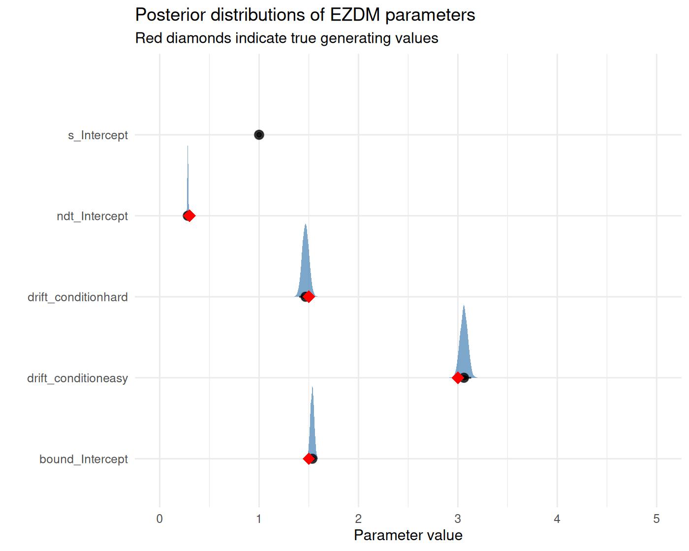
6 Comparing conditions
As bmm feeds seamlessly into brms, we can use Bayesian hypothesis testing via Savage-Dickey density ratios to compare drift rates between conditions:
# Test if drift rate is higher in easy vs hard condition
brms::hypothesis(fit, "exp(drift_conditioneasy) > exp(drift_conditionhard)")
#> Hypothesis Tests for class b:
#>                 Hypothesis Estimate Est.Error CI.Lower CI.Upper Evid.Ratio
#> 1 (exp(drift_condit... > 0     1.59      0.04     1.52     1.66        Inf
#>   Post.Prob Star
#> 1         1    *
#> ---
#> 'CI': 90%-CI for one-sided and 95%-CI for two-sided hypotheses.
#> '*': For one-sided hypotheses, the posterior probability exceeds 95%;
#> for two-sided hypotheses, the value tested against lies outside the 95%-CI.
#> Posterior probabilities of point hypotheses assume equal prior probabilities.