Distribution functions for the Signal Discrimination Model (SDM)

Density, distribution function, and random generation for the Signal Discrimination Model (SDM) Distribution with location mu, memory strength c, and precision kappa. Currently only a single activation source is supported.

Usage

dsdm(x, mu = 0, c = 3, kappa = 3.5, log = FALSE, parametrization = "sqrtexp")

psdm(
  q,
  mu = 0,
  c = 3,
  kappa = 3.5,
  lower.tail = TRUE,
  log.p = FALSE,
  lower.bound = -pi,
  parametrization = "sqrtexp"
)

qsdm(p, mu = 0, c = 3, kappa = 3.5, parametrization = "sqrtexp")

rsdm(n, mu = 0, c = 3, kappa = 3.5, parametrization = "sqrtexp")

Arguments

x

Vector of quantiles

mu

Vector of location values in radians

c

Vector of memory strength values

kappa

Vector of precision values

log

Logical; if TRUE, values are returned on the log scale.

parametrization

Character; either "bessel" or "sqrtexp" (default). See the online article for details on the parameterization.

q

Vector of quantiles

lower.tail

Logical; If TRUE (default), return P(X <= x). Else, return P(X > x)

log.p

Logical; if TRUE, probabilities are returned on the log scale.

lower.bound

Numeric; Lower bound of integration for the cumulative distribution

p

Vector of probabilities

n

Number of observations to sample

Value

dsdm gives the density, psdm gives the distribution function, qsdm gives the quantile function, rsdm generates random deviates, and .dsdm_integrate is a helper function for calculating the density of the SDM distribution.

Details

Parametrization

See the online article for details on the parameterization. Oberauer (2023) introduced the SDM with the bessel parametrization. The sqrtexp parametrization is the default in the bmm package for numerical stability and efficiency. The two parametrizations are related by the functions c_bessel2sqrtexp() and c_sqrtexp2bessel().

The cumulative distribution function

Since responses are on the circle, the cumulative distribution function requires you to choose a lower bound of integration. The default is \(-\pi\), as for the brms::pvon_mises() function but you can choose any value in the argument lower_bound of psdm. Another useful choice is the mean of the response distribution minus \(\pi\), e.g. lower_bound = mu-pi. This is the default in circular::pvonmises(), and it ensures that 50% of the cumulative probability mass is below the mean of the response distribution.

References

Oberauer, K. (2023). Measurement models for visual working memory - A factorial model comparison. Psychological Review, 130(3), 841–852

Examples

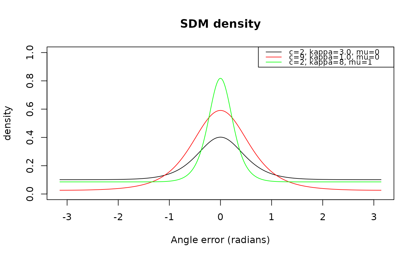
# plot the density of the SDM distribution
x <- seq(-pi,pi,length.out=10000)
plot(x,dsdm(x,0,2,3),type="l", xlim=c(-pi,pi),ylim=c(0,1),
     xlab="Angle error (radians)",
     ylab="density",
     main="SDM density")
lines(x,dsdm(x,0,9,1),col="red")
lines(x,dsdm(x,0,2,8),col="green")
legend("topright",c("c=2, kappa=3.0, mu=0",
                    "c=9, kappa=1.0, mu=0",
                    "c=2, kappa=8, mu=1"),
       col=c("black","red","green"),lty=1, cex=0.8)


# plot the cumulative distribution function of the SDM distribution
p <- psdm(x, mu = 0, c = 3.1, kappa = 5)
plot(x,p,type="l")


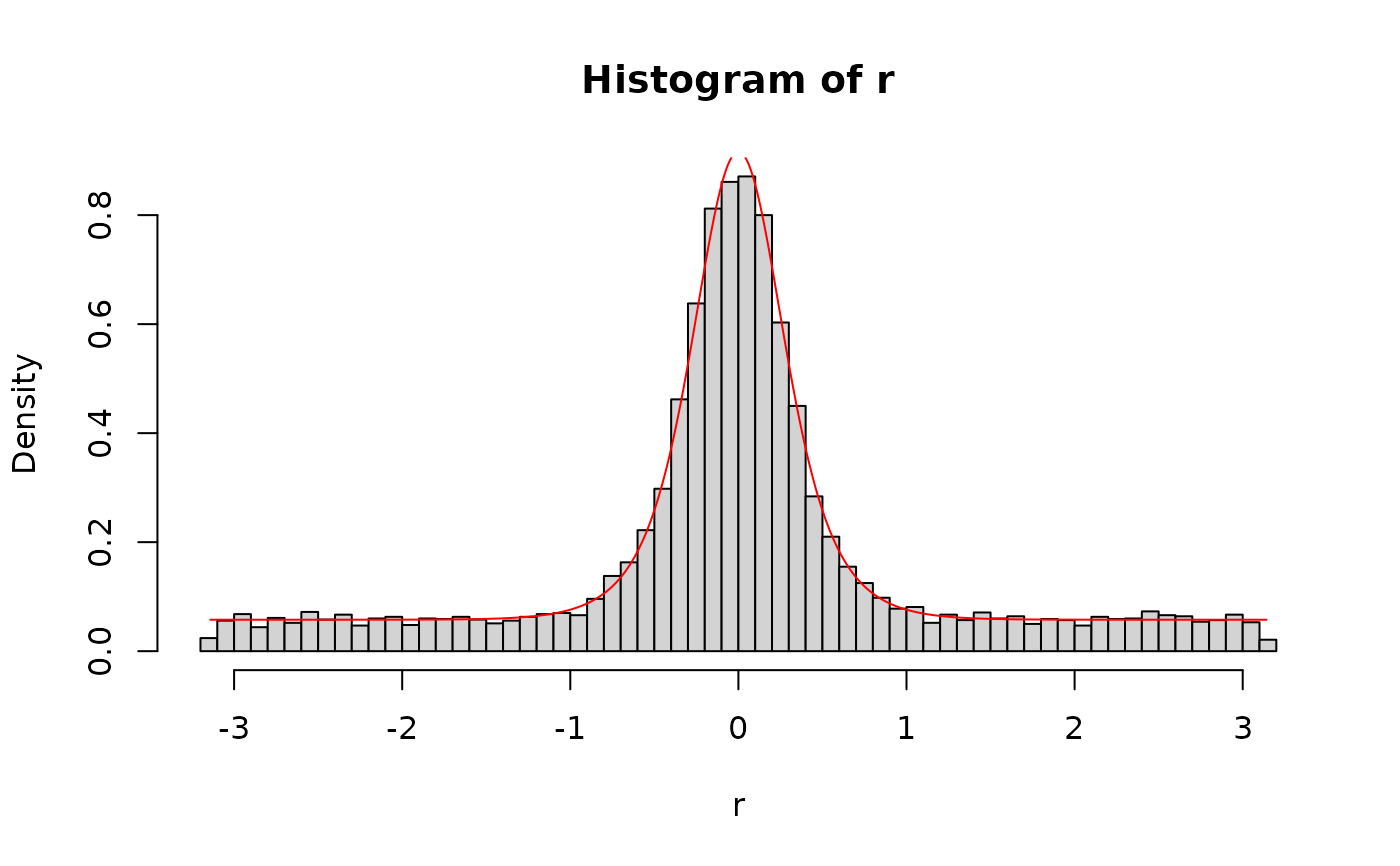
# generate random deviates from the SDM distribution and overlay the density
r <- rsdm(10000, mu = 0, c = 3.1, kappa = 5)
d <- dsdm(x, mu = 0, c = 3.1, kappa = 5)
hist(r, breaks=60, freq=FALSE)
lines(x,d,type="l", col="red")