Mixture models for visual working memory
Ven Popov
Gidon Frischkorn
Source:vignettes/mixture_models.Rmd
mixture_models.Rmd1 Introduction to the models
The two-parameter mixture model (Zhang and Luck 2008) and the three-parameter mixture model (Bays, Catalao, and Husain 2009) are measurement models for continuous reproduction tasks in the visual working memory domain (for details on the task, see vignette('vwm-crt')). As other measurement models for continuous reproduction tasks, their goal is to model the distribution of angular response errors.
The two-parameter mixture model (?mixture2p) distinguishes two memory states that lead to responses with a mixture of two different distributions of angular errors. The two states are:
having a representation of the cued object with a certain precision of its feature in visual working memory (solid blue distribution in Figure 1.1)
having no representation in visual working memory and thus guessing a random response (dashed red distribution).
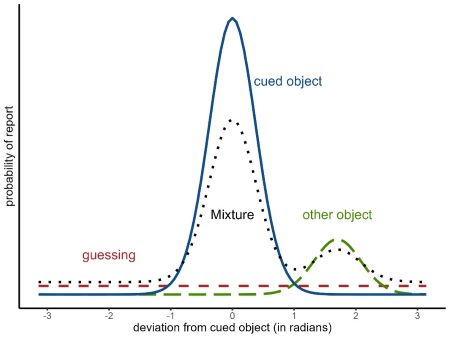
Figure 1.1: Mixtures of response distributions
Responses based on a noisy memory representation of the correct feature come from a circular normal distribution (i.e., von Mises) centered on the correct feature value, while guessing responses come from a uniform distribution along the entire circle:
\[ p(\theta) = p_{mem} \cdot \text{vM}(\theta; \mu, \kappa) + (1-p_{mem}) \cdot \text{Uniform}(\theta; -\pi, \pi) \\ \] \[ p_{guess} = 1-p_{mem} \\ \] \[ vM(\theta; \mu, \kappa) = \frac{e^{\kappa \cos(\theta - \mu)}}{2\pi I_0(\kappa)} \]
where \(\theta\) is the response angle, \(p_{mem}\) is the probability that responses come from memory of target feature, \(\mu\) is the mean of the von Mises distribution representing the target feature, and \(\kappa\) is the concentration parameter of the von Mises distribution, representing the precision of the target memory representation.
The three-parameter mixture model (?mixture3p) adds a third state: confusing the cued object with another object shown during encoding and thus reporting the feature of the other object (long dashed green distribution in Figure 1.1). Responses from this state are sometimes called non-target responses or swap errors. The non-target responses also come from a von Mises distribution centered on the feature of the non-target object. The probability of non-target responses is represented by the parameter \(p_{nt}\), and the complete model is:
\[ p(\theta) = p_{mem} \cdot \text{vM}(\theta; \mu_t, \kappa) + p_{nt} \cdot \frac{\sum_{i=1}^{n} \text{vM}(\theta; \mu_{i}, \kappa)}{n} + (1-p_{mem}-p_{nt}) \cdot \text{Uniform}(\theta; -\pi, \pi) \\ \] \[ p_{guess} = 1-p_{mem}-p_{nt} \]
where \(\mu_{t}\) is the location of the target feature, \(\mu_{i}\) is the location of the i-th non-target feature, \(n\) is the number of non-target features.
In most applications of the model, the responses are coded as the angular error relative to the target feature. The same is true for the non-target memory representations, which are assumed to be centered on the target feature, and the precision of the non-target memory representation is assumed to be the same as the precision of the target memory representation. This is the version of the model implemented in the bmm package:
\[ p(\theta) = p_{mem} \cdot \text{vM}(\theta; 0, \kappa) + p_{nt} \cdot \frac{\sum_{i=1}^{n} \text{vM}(\theta; \mu_{i}-\mu_t, \kappa)}{n} + (1-p_{mem}-p_{nt}) \cdot \text{Uniform}(\theta; -\pi, \pi) \]
2 The data
Begin by loading the bmm package:
library(bmm)
#> Loading required package: brms
#> Loading required package: Rcpp
#> Loading 'brms' package (version 2.20.4). Useful instructions
#> can be found by typing help('brms'). A more detailed introduction
#> to the package is available through vignette('brms_overview').
#>
#> Attaching package: 'brms'
#> The following object is masked from 'package:stats':
#>
#>     ar
For this example, we will analyze data from Bays, Catalao, and Husain (2009). The data is included in the mixtur R package and can be loaded with the following command:
# install the mixtur package if you haven't done so
# install.packages("mixtur")
dat <- mixtur::bays2009_full
The data contains the following columns:
| id | set_size | duration | response | target | non_target_1 | non_target_2 | non_target_3 | non_target_4 | non_target_5 | |
|---|---|---|---|---|---|---|---|---|---|---|
| 321 | 1 | 4 | 2000 | 0.846 | 0.100 | 3.025 | -0.665 | 2.054 | NA | NA |
| 322 | 1 | 4 | 2000 | -1.634 | -0.845 | 2.985 | 2.633 | 2.103 | NA | NA |
| 323 | 1 | 4 | 100 | -1.684 | -1.951 | 0.312 | -1.924 | 0.622 | NA | NA |
| 324 | 1 | 4 | 100 | 0.713 | 0.133 | 1.502 | 3.089 | -0.958 | NA | NA |
| 325 | 1 | 4 | 2000 | 1.317 | 1.439 | -2.675 | -1.191 | 1.970 | NA | NA |
| 326 | 1 | 4 | 2000 | -1.316 | -0.384 | 0.845 | 0.274 | -0.465 | NA | NA |
where:
-
idis a unique identifier for each participant -
setsizeis the number of items presented in the memory array -
responsethe participant’s recollection of the target orientation in radians -
targetthe feature value of the target in radians -
non_target_1tonon_target5are the feature values of the non-targets in radians
The trials vary in set_size (1, 2, 3 or 6), and also vary in encoding duration.
To fit the mixture models with bmm, first we have to make sure that the data is in the correct format. The response variable should be in radians and represent the angular error relative to the target, and the non-target variables should be in radians and be centered relative to the target. You can find these requirements in the help topic for ?mixture2p and ?mixture3p.
In this dataset, the response and non-target variables are already in radians, but they is not centered relative to the target. We can check that by plotting the response distribution. Because memory items are selected at random on each trial, the non-centered responses show a uniform distribution:
library(ggplot2)
ggplot(dat, aes(response)) +
  geom_histogram(binwidth = 0.5, fill = "lightblue", color = "black") +
  labs(title = "Response distribution", x = "Response error (radians)", y = "Frequency")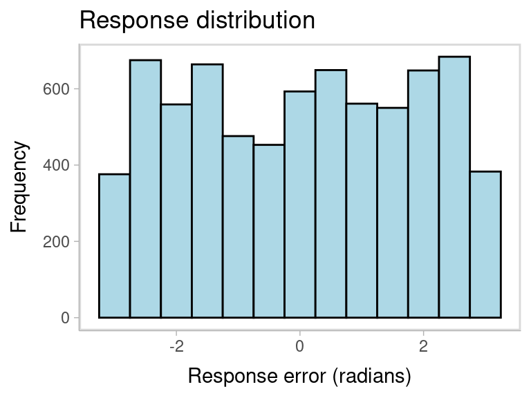
We can center the response and non-target variables by subtracting the target value from them. We can do this with the mutate function from the dplyr package. We also need to make sure that the response is in the range of \((-\pi, \pi)\), and the non-target variables are in the range of \((-\pi, \pi)\). We can do this with the wrap function from the bmm package. As we can see from the new plot, the response distribution is now centered on 0.
library(dplyr)
dat_preprocessed <- dat %>%
  mutate(error = wrap(response - target),
         non_target_1 = wrap(non_target_1 - target),
         non_target_2 = wrap(non_target_2 - target),
         non_target_3 = wrap(non_target_3 - target),
         non_target_4 = wrap(non_target_4 - target),
         non_target_5 = wrap(non_target_5 - target),
         set_size = as.factor(set_size))

ggplot(dat_preprocessed, aes(error)) +
  geom_histogram(bins=60, fill = "lightblue", color = "black") +
  labs(title = "Response distribution", x = "Response error (radians)", y = "Frequency") +
  facet_wrap(~set_size)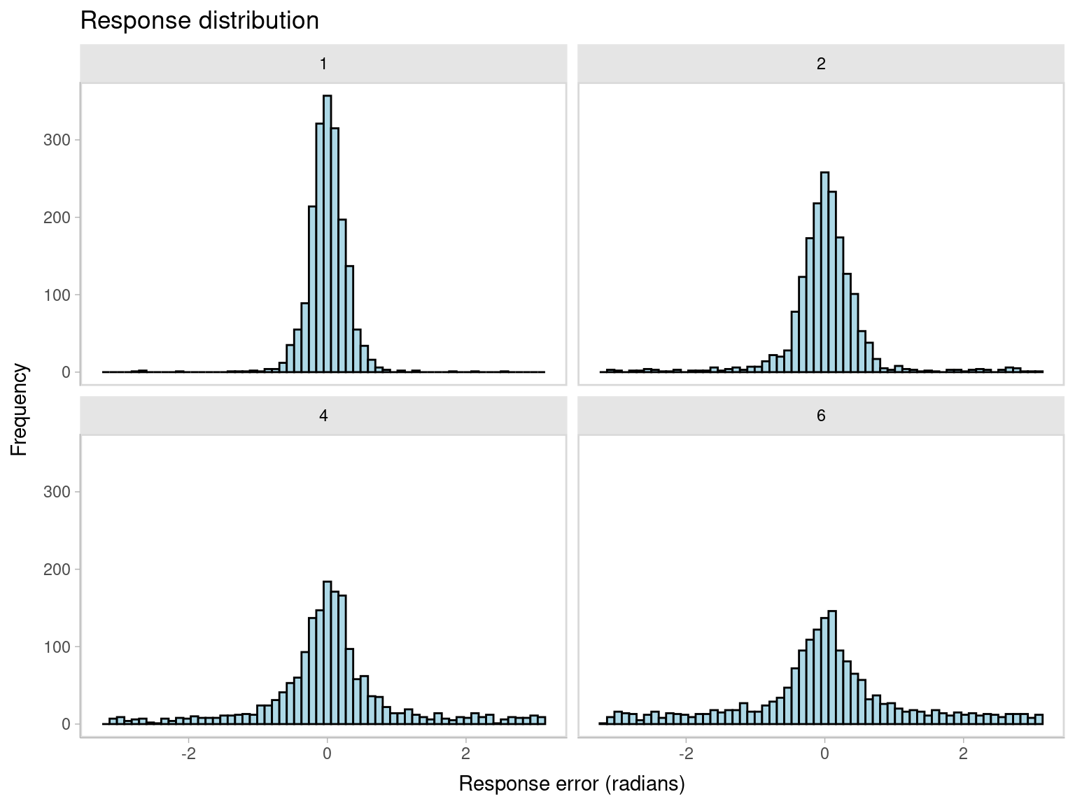
From the plot above we can also see that performace gets substantially worse with increasing set size. Now, we can fit the two mixture models two understand what is driving this pattern.
3 Fitting the 2-parameter mixture model with bmm
To fit the two-parameter mixture model, we need to specify the model formula and the model. For the model formula we use the brms package’s bf function.
For all linear model formulas in brms, the left side of an equation refers to the to-be predicted variable or parameter and the right side specifies the variables used to predict it.
In this example, we want to fit a model in which both the probability of memory responses and the precision of the memory responses vary with set size. We also want the effect of set size to vary across participants.
The model formula has three components:
- The response variable
erroris predicted by a constant term, which is internally fixed to have a mean of 0 - The precision parameter
kappais predicted by set size, and the effect of set size varies across participants - The mixture weight1 for memory responses
thetatis predicted by set size, and the effect of set size varies across participants.
ff <- bmmformula(thetat ~ 0 + set_size + (0 + set_size | id),
                 kappa ~ 0 + set_size + (0 + set_size | id))
Then we specify the model as simply as:
model <- mixture2p(resp_err = "error")Finally, we fit the model with the fit_model function. The fit model function uses
the brms package to fit the model, so you can pass to it any argument that you would pass to the brm function.
fit <- fit_model(
  formula = ff,
  data = dat_preprocessed,
  model = model,
  parallel=T,
  iter=2000,
  refresh=100,
  backend='cmdstanr'
)
4 Results of the 2-parameter mixture model
We can now inspect the model fit:
summary(fit)
#>  Family: mixture(von_mises, von_mises)
#>   Links: mu1 = tan_half; kappa1 = log; mu2 = tan_half; kappa2 = log; theta1 = identity; theta2 = identity
#> Formula: error ~ 1
#>          mu1 ~ 1
#>          kappa ~ 0 + set_size + (0 + set_size | id)
#>          thetat ~ 0 + set_size + (0 + set_size | id)
#>          kappa2 ~ 1
#>          mu2 ~ 1
#>          kappa1 ~ kappa
#>          theta1 ~ thetat
#>    Data: .x2 (Number of observations: 7271)
#>   Draws: 4 chains, each with iter = 2000; warmup = 1000; thin = 1;
#>          total post-warmup draws = 4000
#>
#> Group-Level Effects:
#> ~id (Number of levels: 12)
#>                                        Estimate Est.Error l-95% CI u-95% CI Rhat Bulk_ESS Tail_ESS
#> sd(kappa_set_size1)                        0.34      0.09     0.21     0.55 1.00     1368     2540
#> sd(kappa_set_size2)                        0.22      0.07     0.10     0.38 1.00     2143     2214
#> sd(kappa_set_size4)                        0.35      0.11     0.18     0.62 1.00     1914     2637
#> sd(kappa_set_size6)                        0.38      0.13     0.18     0.70 1.00     2155     2110
#> sd(thetat_set_size1)                       0.66      0.47     0.05     1.78 1.00     1238     1214
#> sd(thetat_set_size2)                       0.85      0.25     0.48     1.43 1.00     1893     2665
#> sd(thetat_set_size4)                       0.83      0.22     0.50     1.36 1.00     2100     2965
#> sd(thetat_set_size6)                       0.60      0.16     0.36     0.99 1.00     2016     2843
#> cor(kappa_set_size1,kappa_set_size2)       0.68      0.22     0.11     0.96 1.00     2456     2681
#> cor(kappa_set_size1,kappa_set_size4)       0.39      0.29    -0.23     0.86 1.00     2208     2598
#> cor(kappa_set_size2,kappa_set_size4)       0.28      0.34    -0.43     0.85 1.00     1552     2585
#> cor(kappa_set_size1,kappa_set_size6)       0.45      0.29    -0.19     0.90 1.00     1767     1953
#> cor(kappa_set_size2,kappa_set_size6)       0.48      0.30    -0.20     0.93 1.00     1665     2209
#> cor(kappa_set_size4,kappa_set_size6)       0.49      0.30    -0.19     0.92 1.00     2549     3424
#> cor(thetat_set_size1,thetat_set_size2)     0.38      0.38    -0.51     0.91 1.01      811      891
#> cor(thetat_set_size1,thetat_set_size4)     0.25      0.38    -0.56     0.86 1.01      674      867
#> cor(thetat_set_size2,thetat_set_size4)     0.57      0.25    -0.02     0.94 1.00     1465     2404
#> cor(thetat_set_size1,thetat_set_size6)     0.22      0.37    -0.59     0.82 1.01      858      948
#> cor(thetat_set_size2,thetat_set_size6)     0.65      0.22     0.11     0.95 1.00     2192     3272
#> cor(thetat_set_size4,thetat_set_size6)     0.68      0.21     0.14     0.95 1.00     2687     3137
#>
#> Population-Level Effects:
#>                  Estimate Est.Error l-95% CI u-95% CI Rhat Bulk_ESS Tail_ESS
#> mu1_Intercept        0.00      0.00     0.00     0.00   NA       NA       NA
#> mu2_Intercept        0.00      0.00     0.00     0.00   NA       NA       NA
#> kappa2_Intercept  -100.00      0.00  -100.00  -100.00   NA       NA       NA
#> kappa_set_size1      2.89      0.10     2.68     3.11 1.00     1040     1459
#> kappa_set_size2      2.39      0.08     2.24     2.54 1.00     1678     1810
#> kappa_set_size4      2.06      0.12     1.82     2.32 1.00     1797     2254
#> kappa_set_size6      1.94      0.14     1.66     2.22 1.00     2167     2474
#> thetat_set_size1     4.49      0.38     3.81     5.33 1.00     2450     2196
#> thetat_set_size2     2.57      0.30     1.99     3.18 1.00     1461     1931
#> thetat_set_size4     1.05      0.26     0.53     1.59 1.00     1553     1798
#> thetat_set_size6     0.27      0.19    -0.12     0.66 1.00     1591     1859
#>
#> Draws were sampled using sample(hmc). For each parameter, Bulk_ESS
#> and Tail_ESS are effective sample size measures, and Rhat is the potential
#> scale reduction factor on split chains (at convergence, Rhat = 1).
The summary shows the estimated fixed effects for the precision and the mixture weight, as well as the estimated random effects for the precision and the mixture weight. All Rhat values are close to 1, which is a good sign that the chains have converged. The effective sample sizes are also high, which means that the chains have mixed well.
We now want to understand the estimated parameters.
-
kappais coded withinbrmswith a log-link function, so we need to exponentiate the estimates to get the precision parameter. We can further use thek2sdfunction to convert the precision parameter to the standard deviation units. -
thetatis the mixture weight for memory responses. As described in footnote 1, we can use the softmax function to get the probability of memory responses.
# extract the fixed effects from the model and determine the rows that contain
# the relevant parameter estimates
fixedEff <- brms::fixef(fit)
thetat <- fixedEff[grepl("thetat",rownames(fixedEff)),]
kappa <- fixedEff[grepl("kappa_",rownames(fixedEff)),]

# transform parameters because brms uses special link functions
kappa <- exp(kappa)
sd <- k2sd(kappa[,1])
pmem <- exp(thetat)/(exp(thetat)+1)
pg <- exp(0)/(exp(thetat)+1)
Our estimates for kappa over setsize are:
kappa
#>                  Estimate Est.Error      Q2.5     Q97.5
#> kappa_set_size1 18.071106  1.109868 14.621540 22.350820
#> kappa_set_size2 10.952056  1.077957  9.407307 12.670849
#> kappa_set_size4  7.834605  1.131517  6.170123 10.155392
#> kappa_set_size6  6.950459  1.149041  5.273423  9.221514
Standard deviation:
names(sd) <- paste0("Set size ", c(1,2,4,6))
round(sd,3)
#> Set size 1 Set size 2 Set size 4 Set size 6
#>      0.239      0.310      0.370      0.395
Probability that responses comes from memory:
rownames(pmem) <- paste0("Set size ", c(1,2,4,6))
round(pmem,3)
#>            Estimate Est.Error  Q2.5 Q97.5
#> Set size 1    0.989     0.593 0.978 0.995
#> Set size 2    0.929     0.574 0.880 0.960
#> Set size 4    0.740     0.565 0.629 0.830
#> Set size 6    0.566     0.548 0.471 0.659
It is even better to visualize the entire posterior distribution of the parameters.
library(tidybayes)
library(tidyr)

# extract the posterior draws
draws <- tidybayes::tidy_draws(fit)
draws_theta <- select(draws, b_thetat_set_size1:b_thetat_set_size6)
draws_kappa <- select(draws, b_kappa_set_size1:b_kappa_set_size6)

# transform parameters because brms uses special link functions
draws_theta <- exp(draws_theta)/(exp(draws_theta) + 1)
draws_kappa <- exp(draws_kappa)

# plot posterior
as.data.frame(draws_theta) %>%
  gather(par, value) %>%
  mutate(par = gsub("b_thetat_set_size", "", par)) %>%
  ggplot(aes(par, value)) +
  tidybayes::stat_halfeyeh(normalize = "groups", orientation = "vertical") +
  labs(y = "Probability of memory response", x = "Set size", parse = TRUE)

as.data.frame(draws_kappa) %>%
  gather(par, value) %>%
  mutate(value = k2sd(value)) %>%
  mutate(par = gsub("b_kappa_set_size", "Set size ", par)) %>%
  ggplot(aes(par,value)) +
  tidybayes::stat_halfeyeh(normalize = "groups", orientation = "vertical") +
  labs(y = "Memory imprecision (SD)", x = "Set size", parse = TRUE)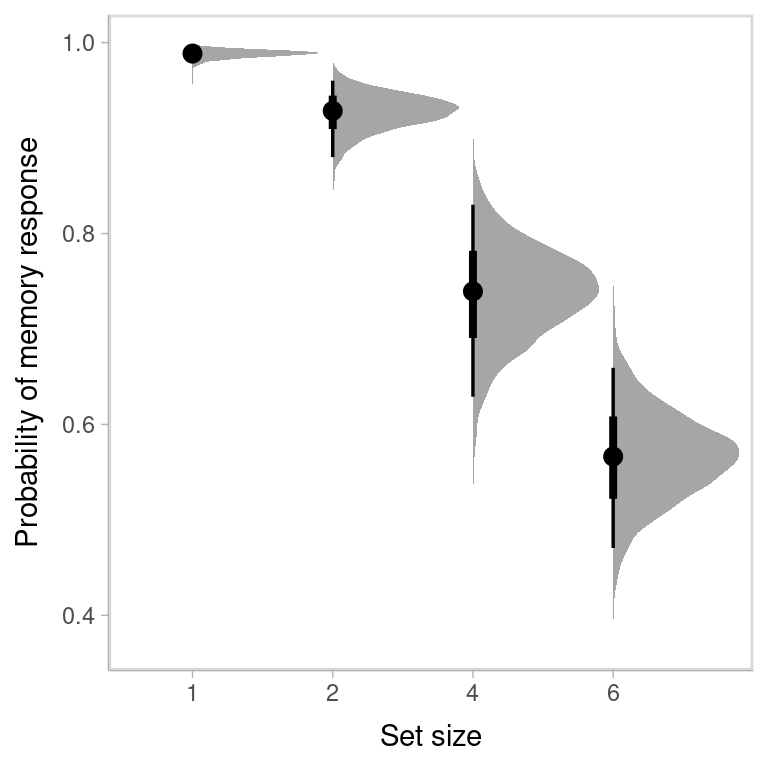
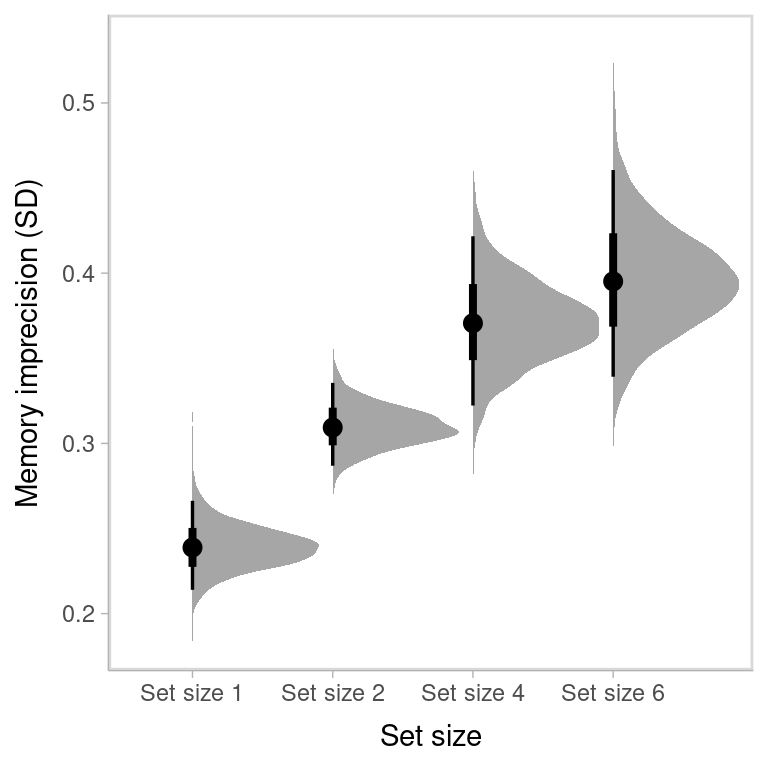
where the black dot represents the median of the posterior distribution, the thick line represents the 50% credible interval, and the thin line represents the 95% credible interval.
5 Fitting the 3-parameter mixture model with bmm
Fitting the 3-parameter mixture model is very similar. We have an extra parameter thetant that represents the mixture weight for non-target responses2. We also need to specify the names of the non-target variables and the setsize3 variable in the mixture3p function.
ff <- bmf(
  thetat ~ 0 + set_size + (0 + set_size | id),
  thetant ~ 0 + set_size + (0 + set_size | id),
  kappa ~ 0 + set_size + (0 + set_size | id)
)

model <- mixture3p(resp_err = "error", nt_features = paste0('non_target_',1:5), setsize = 'set_size')
Then we run the model just like before:
fit3p <- fit_model(
  formula = ff,
  data = dat_preprocessed,
  model = model,
  parallel=T,
  iter=2000,
  refresh=100,
  backend='cmdstanr'
)
The rest of the analysis is the same as for the 2-parameter model. We can inspect the model fit, extract the parameter estimates, and visualize the posterior distributions.
In the above example we specified all column names for the non_targets explicitely via paste0('non_target_',1:5). Alternatively, you can use a regular expression to match the non-target feature columns in the dataset. This is useful when the non-target feature columns are named in a consistent way, e.g. non_target_1, non_target_2, non_target_3, etc. For example, you can specify the model a few different ways via regular expressions: