The Interference Measurement Model (IMM)
Gidon Frischkorn
Ven Popov
Source:vignettes/articles/bmm_imm.Rmd
bmm_imm.Rmd1 Introduction to the model
The Interference Measurement Model (IMM) is a measurement model for continous reproduction tasks in the domain of visual working memory. The model was introduced by Oberauer et al. (2017) . The aim of the IMM is to capture the response behavior in continuous reproduction tasks including the occurrence of swap errors to other items encoded in visual working memory.
The IMM assumes that during retrieval, to-be-remembered items or features (e.g., colors, orientations, or shapes) are associated with the context they appeared in (e.g. the spatial location). These associations can be continuous in their strength and represent bindings between the contents and context of to-be-remembered information (see Figure 1.1). At retrieval there are different sources of activation that contribute to the activation of the to-be-retrieved contents. Background noise (b) uniformly activates all possible responses, for example all 360 colors that participants can chose from in a color wheel experiment. Cue-independent activation (a) equally activates all features that were encoded into visual working memory during retrieval. And cue-dependent activation (c) activates the features that are associated with the current retrieval cue (e.g., the spatial location cued to be retrieved). Additionally, the IMM assumes that cue-dependent activation follows a generalization gradient (s) that activates similar contexts.
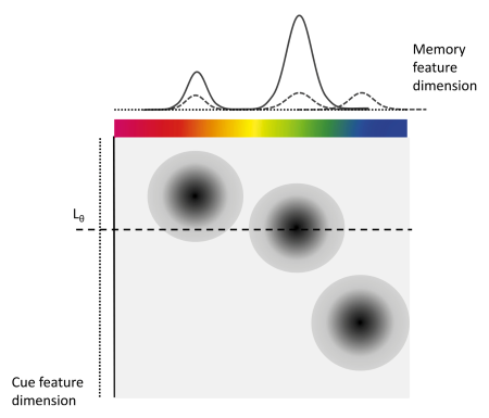
Figure 1.1: Illustration of the IMM from Oberauer et al. (2017)
The activation for each potential feature \(x\) that could be retrieved is the sum of the weighted activation from all three activation sources, given a retrieval cue \(L\) at the location \(\theta\):
\[ A(x|L_\theta) = b \times A_b(x) + a \times A_a(x) + c \times A_c(c|L_\theta) \]
The background activation (\(A_b\)) is independent from all encoded features and thus modeled as a uniform distribution around the circular feature space. This is implemented as a von-Mises (vM) distribution centered on 0 with a precision \(\kappa = 0\):
\[ A_b(x) = vM(x,0,0) \]
The cue-independent activation (\(A_a\)) is modeled as the sum of von Mises distributions centered on the feature values \(x_i\) of all \(n\) encoded items \(i\) with the precision of memory :
\[ A_a(x) = \sum^n_{i = 1} vM(x,x_i,\kappa) \]
The cue-dependent activation (\(A_c\)) is again modeled as the sum of von Mises distributions centered on the feature values \(x_i\) of all \(n\) encoded items \(i\) with the precision of memory . These distributions are weighted by the spatial distance \(D\) between the context \(L\) a feature was associated with to the cue context \(L_\theta\). This distance is weighted by the generalization gradient \(s\) that captures the specificity of bindings to the cue dimension:
\[ A_c(x|L_\theta) = \sum^n_{i = 1} e^{-s*D(L,L\theta)} \times vM(x,x_i,\kappa) \]
The probability for choosing each response \(\hat{x}\) then results from normalizing the activation for all possible responses \(N\). In the original publication of the IMM this was done using Luce’s choice rule:
\[ P(\hat{x}|L_\theta) = \frac{A(\hat{x}|L_\theta)}{\sum^N_{j=1}A(j|L_\theta)} \]
The bmm package uses the same parameterization, except that it uses a log Link function for all activation parameters to ensure that these parameters are positive.
In sum, the IMM assumes that responses in continuous reproduction tasks are the results of cue-based retrieval and cue-independent activation of all features corrupted by background noise.
2 Parametrization in the bmm package
For identification, one of the weighting parameters has to be fixed. In the original publication the strength of cue-dependent activation \(c\) was fixed to one. The default setup of brms however currently only allows to fix the strength of the background noise \(b\) to one Therefore, in all implementations of the IMM in the bmm package, the strength of cue-dependent and cue-independent activation, \(c\) and \(a\), can be estimated and predicted by independent variables.
Apart from that, both the precision of memory representations \(\kappa\) and the generalization gradient \(s\) are parameterized the same way as in the original publication. Please also note, that the scaling of the generalization gradient s is dependent on the scaling of the distance D between the target location and the locations of the non-targets. In previous studies estimating the IMM (Oberauer et al. 2017) these distances were scaled in radians, as all items were placed on a imaginary circle around the center of the screen. However, other studies might position the color patches randomly inside a frame of a certain width and height and thus might use euclidean distances. Also changing the radius of the imaginary circles that color patches are placed on, will change the absolute distance between items. This will affect the absolute size of the generalization gradient s. Thus, differences in the generalization gradient s between different studies should not be interpreted strongly, especially if the studies used different distance measures or different experimental settings with respect to the placement of the items. For now, we recommend that only differences in the generalization gradient s between conditions of a single experiment should be taken as robust results.
3 Fitting the model with bmm
You should start by loading the bmm package:
3.1 Generating simulated data
Should you already have a data set you want to fit, you can skip this section. Alternatively, you can use data provided with the package (see data(package='bmm')) or generate data using the random generation function provided in the bmm package.
# set seed for reproducibility
set.seed(123)

# specfiy generating parameters
Cs <- c(4,4,2,2)
As <- c(0.5,1,0.5,0.5)
Ss <- c(10,10,5,5)
kappas <- c(15,10,15,10)
nTrials = 2000
set_size = 5

simData <- data.frame()
for (i in 1:length(Cs)) {
  # generate different non-target locations for each condition
  item_location <- c(0, runif(set_size - 1, -pi,pi))

  # generate different distances for each condition
  item_distance <- c(0, runif(set_size - 1, min = 0.1, max = pi))

  # simulate data for each condition
  genData <- rimm(n = nTrials,
                  mu = item_location,
                  dist = item_distance,
                  c = Cs[i], a = As[i],
                  b = 1, s = Ss[i], kappa = kappas[i])

  condData <- data.frame(
    resp_error = genData,
    trialID = 1:nTrials,
    cond = i,
    color_item1 = 0,
    dist_item1 = 0
  )

  init_colnames <- colnames(condData)

  for (j in 1:(set_size - 1)) {
    condData <- cbind(condData,item_location[j + 1])
    condData <- cbind(condData,item_distance[j + 1])
  }

  colnames(condData) <- c(init_colnames,
                          paste0(rep(c("color_item","dist_item"),times = set_size - 1),
                                 rep(2:(set_size),each = 2)))

  simData <- rbind(simData,condData)
}

# convert condition variable to a factor

simData$cond <- as.factor(simData$cond)
3.2 Estimating the model with bmm
To estimate the IMM we first need to specify a formula. We specify the formula using the bmmformula function (or bmf). In this formula, we directly estimate all parameters for each of the four conditions. Unlike for brmsformula we do not provide the dependent variable in this formula.:
model_formula <- bmf(
  c ~ 0 + cond,
  a ~ 0 + cond,
  s ~ 0 + cond,
  kappa ~ 0 + cond
)
Then, we can specify the model that we want to estimate. This includes specifying the name of the variable containing the dependent variable resp_error in our simulated data set. Additionally, we also need to provide the information of the non_target locations, the name of the variable coding the spatial distances of the nt_features to the target spaDist, and the set_size used in our data. The set_size can either be a fixed integer, if there is only one set_size in your data, or the name of the variable coding the set_size in your data:
model <- imm(resp_error = "resp_error",
             nt_features = paste0("color_item",2:5),
             set_size = set_size,
             nt_distances = paste0("dist_item",2:5),
             version = "full")
In the above example we specified all column names for the non_targets explicitly via paste0('color_item',2:5). Alternatively, you can use a regular expression to match the non-target feature columns in the dataset. For example, you can specify the model a few different ways via regular expressions:
model <- imm(resp_error = "resp_error",
             nt_features = "color_item[2-5]",
             set_size = set_size,
             nt_distances = "dist_item[2-5]",
             regex = TRUE)
By default the imm() function implements the full imm model. You can specify a reduced model by setting the version argument to “abc” or “bsc” (see ?imm).
Finally, we can fit the model by passing all the relevant arguments to the bmm() function:
fit <- bmm(
  formula = model_formula,
  data = simData,
  model = model,
  cores = 4,
  backend = "cmdstanr",
  file = "assets/bmmfit_imm_vignette"
)
Running this model takes about 2 to 5 minutes (depending on the speed of your computer). We specified the file argument to save the model fit and avoid reruning the model in the future, but this line is optional. Both brms and cmdstanr typically print out some information on the sampling progress.
Using this fit object we can have a quick look at the summary of the fitted model:
summary(fit) Model: imm(resp_error = "resp_error",
nt_features = paste0("color_item", 2:5),
nt_distances = paste0("dist_item", 2:5),
set_size = set_size)
Links: mu1 = tan_half; kappa = log; a = log; c = log; s = log
Formula: mu1 = 0
kappa ~ 0 + cond
a ~ 0 + cond
c ~ 0 + cond
s ~ 0 + cond
Data: simData (Number of observations: 8000)
Draws: 4 chains, each with iter = 2000; warmup = 1000; thin = 1;
total post-warmup draws = 4000
Regression Coefficients:
Estimate Est.Error l-95% CI u-95% CI Rhat Bulk_ESS Tail_ESS
kappa_cond1 2.66 0.05 2.56 2.77 1.00 4057 2739
kappa_cond2 2.46 0.06 2.34 2.57 1.00 4242 2685
kappa_cond3 2.76 0.06 2.63 2.89 1.00 3797 2534
kappa_cond4 2.27 0.06 2.15 2.38 1.00 4886 2930
a_cond1 -0.80 0.24 -1.44 -0.44 1.00 2422 1245
a_cond2 0.08 0.19 -0.27 0.46 1.00 3358 2847
a_cond3 -0.89 0.15 -1.20 -0.59 1.00 3065 2508
a_cond4 -0.64 0.16 -0.96 -0.32 1.00 3707 3062
c_cond1 1.40 0.10 1.20 1.61 1.00 4138 2634
c_cond2 1.25 0.17 0.93 1.59 1.00 3185 2931
c_cond3 0.64 0.12 0.42 0.87 1.00 3006 2758
c_cond4 0.78 0.12 0.56 1.01 1.00 4198 3187
s_cond1 0.78 0.56 0.08 2.27 1.00 1949 1342
s_cond2 2.27 0.12 2.02 2.52 1.00 4398 2165
s_cond3 1.44 0.44 0.87 2.53 1.00 2179 1899
s_cond4 1.75 0.14 1.52 2.04 1.00 3945 2221
Constant Parameters:
Value
mu1_Intercept 0.00
Draws were sampled using sample(hmc). For each parameter, Bulk_ESS
and Tail_ESS are effective sample size measures, and Rhat is the potential
scale reduction factor on split chains (at convergence, Rhat = 1).
The first thing you might notice is that below the parts of the formula that was passed to the bmm() function, bmm has added a lot of additional specifications to implement the IMM. This is nothing that you have to check. But if you are interested in customizing and exploring different assumptions imposed by the IMM, you could start by taking this formula and adapting it accordingly.
Next, we can have a look at the estimated parameters. The first thing we should check is if the sampling converged, this is indicated by all Rhat values being close to one. If you want to do more inspection of the sampling, you can check out the functionality implemented in brmsto do this.
The parameter estimates for c and a are already on their native scale, but both s and kappa are estimated using a log link function, so we have to transform these back to the native scale.
fixedFX <- brms::fixef(fit)

# print posterior means for the s parameter
fixedFX[startsWith(rownames(fixedFX),"c_"),]
#>          Estimate Est.Error      Q2.5     Q97.5
#> c_cond1 1.4029191 0.1043972 1.2043833 1.6140742
#> c_cond2 1.2515988 0.1666962 0.9340766 1.5871405
#> c_cond3 0.6383213 0.1168157 0.4215037 0.8661965
#> c_cond4 0.7773603 0.1154368 0.5603164 1.0053527

# print posterior means for the s parameter
fixedFX[startsWith(rownames(fixedFX),"a_"),]
#>            Estimate Est.Error       Q2.5      Q97.5
#> a_cond1 -0.80298699 0.2368208 -1.4410525 -0.4400670
#> a_cond2  0.08206161 0.1863355 -0.2718943  0.4588391
#> a_cond3 -0.89235205 0.1513407 -1.1950945 -0.5943169
#> a_cond4 -0.63825173 0.1603443 -0.9612214 -0.3244024

# print posterior means for the s parameter
exp(fixedFX[grepl("s_",rownames(fixedFX)),])
#>         Estimate Est.Error     Q2.5     Q97.5
#> s_cond1 2.172801  1.758737 1.086510  9.658011
#> s_cond2 9.646052  1.132108 7.575980 12.387176
#> s_cond3 4.205237  1.552785 2.380787 12.551168
#> s_cond4 5.767301  1.144775 4.563214  7.725994

# print posterior means for the s parameter
exp(fixedFX[grepl("kappa_",rownames(fixedFX)),])
#>              Estimate Est.Error      Q2.5    Q97.5
#> kappa_cond1 14.346976  1.055983 12.929283 16.01333
#> kappa_cond2 11.648836  1.061680 10.360751 13.05853
#> kappa_cond3 15.762715  1.066499 13.841243 17.91177
#> kappa_cond4  9.655314  1.059530  8.619316 10.81511
These results indicate that all parameters, except for s were well recovered. As already noted by Oberauer et al. (2017), a good recovery of the generalization gradient s requires a lot of data. Thus you might consider opting for the simplified version of the IMM without the s parameter, the imm_abc.
We can illustrate the recovery of the data generating parameters by plotting the full posterior distributions alongside the data generating parameters. For this we need to extract the posterior draws using the tidybayes package and include the data generating parameters into the plots of the posteriors.
library(tidybayes)
library(dplyr)
library(tidyr)
library(ggplot2)

# extract the posterior draws
draws <- tidybayes::tidy_draws(fit)
draws <- select(draws, starts_with("b_")) %>% select(-(1:3)) %>%
  mutate_at(vars(starts_with("b_")),exp)

# plot posterior with original parameters overlayed as diamonds
as.data.frame(draws) %>%
  gather(par, value) %>%
  ggplot(aes(value, par)) +
  tidybayes::stat_halfeyeh(normalize = "groups") +
  geom_point(data = data.frame(par = colnames(draws),
                               value = c(kappas, As, Cs, Ss)),
             aes(value,par), color = "red",
             shape = "diamond", size = 2.5) +
  scale_x_continuous(lim=c(-1.5,20))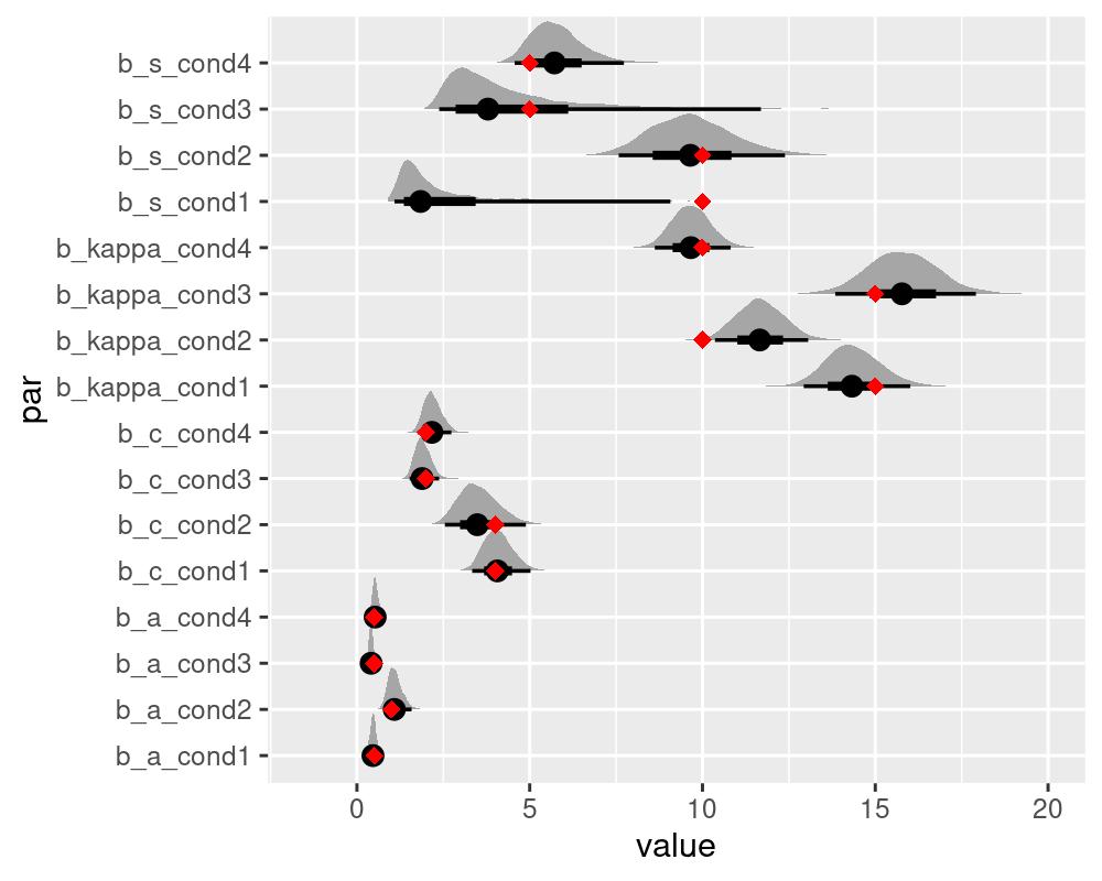
colnames(draws)
#>  [1] "b_kappa_cond1" "b_kappa_cond2" "b_kappa_cond3" "b_kappa_cond4"
#>  [5] "b_a_cond1"     "b_a_cond2"     "b_a_cond3"     "b_a_cond4"
#>  [9] "b_c_cond1"     "b_c_cond2"     "b_c_cond3"     "b_c_cond4"
#> [13] "b_s_cond1"     "b_s_cond2"     "b_s_cond3"     "b_s_cond4"